Hispanopedia Wiki
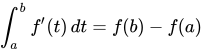
Las distribuciones , también conocidas como distribuciones de Schwartz o funciones generalizadas , son objetos que generalizan la noción clásica de funciones en el análisis matemático . Las distribuciones permiten diferenciar funciones cuyas derivadas no existen en el sentido clásico. En particular, cualquier función localmente integrable tiene una derivada distribucional .
Las distribuciones se utilizan ampliamente en la teoría de ecuaciones diferenciales parciales , donde puede ser más fácil establecer la existencia de soluciones distribucionales ( soluciones débiles ) que de soluciones clásicas , o donde sea apropiado que las soluciones clásicas puedan no existir. Las distribuciones también son importantes en física e ingeniería , donde muchos problemas conducen naturalmente a ecuaciones diferenciales cuyas soluciones o condiciones iniciales son singulares, como la función delta de Dirac .
Normalmente se piensa que una función actúa sobre los puntos del dominio de la función "enviando" un punto del dominio al punto En lugar de actuar sobre puntos, la teoría de la distribución reinterpreta las funciones como si actuaran sobre funciones de prueba de una determinada manera. En aplicaciones a la física y la ingeniería, las funciones de prueba suelen ser funciones complejas (o de valor real ) infinitamente diferenciables con soporte compacto que se definen en algún subconjunto abierto no vacío dado . ( Las funciones de protuberancia son ejemplos de funciones de prueba). El conjunto de todas esas funciones de prueba forma un espacio vectorial que se denota por o


Las funciones más comúnmente encontradas, incluyendo todos los mapas continuos si se usan, pueden reinterpretarse canónicamente como actuando a través de " integración contra una función de prueba". Explícitamente, esto significa que dicha función "actúa sobre" una función de prueba "enviándola" al número que a menudo se denota por Esta nueva acción de define un mapa de valor escalar cuyo dominio es el espacio de funciones de prueba. Esta funcional resulta tener las dos propiedades definitorias de lo que se conoce como una distribución en : es lineal y también es continua cuando se da una cierta topología llamada topología LF canónica . La acción (la integración ) de esta distribución en una función de prueba puede interpretarse como un promedio ponderado de la distribución en el soporte de la función de prueba, incluso si los valores de la distribución en un solo punto no están bien definidos. Distribuciones como esa surgen de funciones de esta manera son ejemplos prototípicos de distribuciones, pero existen muchas distribuciones que no se pueden definir por integración contra ninguna función. Ejemplos de esto último incluyen la función delta de Dirac y distribuciones definidas para actuar mediante la integración de funciones de prueba contra ciertas medidas . No obstante, siempre es posible reducir cualquier distribución arbitraria a una familia más simple de distribuciones relacionadas que surgen a través de tales acciones de integración.





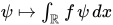


En términos más generales, una distribución en es, por definición, una funcional lineal en que es continua cuando se le da una topología llamada topología LF canónica . Esto conduce al espacio de (todas) las distribuciones en , usualmente denotado por (nótese la prima ), que por definición es el espacio de todas las distribuciones en (es decir, es el espacio dual continuo de ); son estas distribuciones las que constituyen el foco principal de este artículo.


Las definiciones de las topologías adecuadas en los espacios de funciones de prueba y distribuciones se dan en el artículo sobre espacios de funciones de prueba y distribuciones . Este artículo se ocupa principalmente de la definición de distribuciones, junto con sus propiedades y algunos ejemplos importantes.
Historia
El uso práctico de las distribuciones se remonta al uso de las funciones de Green en la década de 1830 para resolver ecuaciones diferenciales ordinarias, pero no se formalizó hasta mucho después. Según Kolmogorov y Fomin (1957), las funciones generalizadas se originaron en el trabajo de Sergei Sobolev (1936) sobre ecuaciones diferenciales parciales hiperbólicas de segundo orden , y las ideas fueron desarrolladas en forma algo ampliada por Laurent Schwartz a fines de la década de 1940. Según su autobiografía, Schwartz introdujo el término "distribución" por analogía con una distribución de carga eléctrica, que posiblemente incluía no solo cargas puntuales sino también dipolos, etc. Gårding (1997) comenta que, aunque las ideas del libro transformador de Schwartz (1951) no eran completamente nuevas, fue el amplio ataque de Schwartz y la convicción de que las distribuciones serían útiles casi en todas partes en el análisis lo que marcó la diferencia.
Notación
A lo largo de este artículo se utilizará la siguiente notación:
- es un entero positivo fijo y es un subconjunto abierto no vacío fijo del espacio euclidiano
- denota los números naturales .
- denotará un número entero no negativo o
- Si es una función entonces denotará su dominio y laEl soporte dedenotado porse define como elcierredel conjuntoen
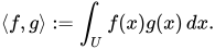
- Para dos funciones, la siguiente notación define un emparejamiento canónico :
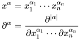
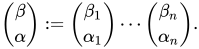
- Un multiíndice de tamaño es un elemento en (dado que es fijo, si se omite el tamaño de los multiíndices, se debe asumir que el tamaño es ). La longitud de un multiíndice se define como y se denota por Los multiíndices son particularmente útiles cuando se trata con funciones de varias variables, en particular, introducimos las siguientes notaciones para un multiíndice dado : También introducimos un orden parcial de todos los multiíndices por si y solo si para todos Cuando definimos su coeficiente binomial de multiíndice como:














Definiciones de funciones de prueba y distribuciones
En esta sección se presentan algunas nociones y definiciones básicas necesarias para definir distribuciones de valores reales en U. En el artículo sobre espacios de funciones de prueba y distribuciones se ofrece un análisis más detallado de las topologías en los espacios de funciones de prueba y distribuciones .
- Dejar
- Sea el espacio vectorial de todas las funciones reales o complejas continuamente diferenciables k veces en U.
- Para cualquier subconjunto compacto, sea y ambos denotan el espacio vectorial de todas aquellas funciones tales que
- Si entonces el dominio de es U y no K . Por lo tanto, aunque depende tanto de K como de U , normalmente solo se indica K . La justificación de esta práctica común se detalla a continuación. La notación solo se utilizará cuando exista riesgo de ambigüedad.
- Cada contiene el mapa constante 0 , incluso si
- Sea el conjunto de todos tales que para algún subconjunto compacto K de U .
- Equivalentemente, es el conjunto de todos los que tienen soporte compacto.
- es igual a la unión de todos los rangos sobre todos los subconjuntos compactos de
- Si es una función de valor real en , entonces es un elemento de si y solo si es una función de protuberancia . Toda función de prueba de valor real en es también una función de prueba de valor complejo en



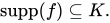



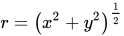
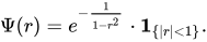


Para todos y cualesquiera subconjuntos compactos de y , tenemos:



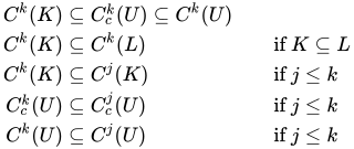

Las distribuciones en U son funcionales lineales continuas en cuando este espacio vectorial está dotado de una topología particular llamada topología LF canónica . La siguiente proposición establece dos condiciones necesarias y suficientes para la continuidad de una función lineal en que a menudo son fáciles de verificar.
Proposición : Una función lineal T en es continua, y por lo tanto una distribución , si y sólo si se cumple cualquiera de las siguientes condiciones equivalentes:
- Para cada subconjunto compacto existen constantes y (dependientes de ) tales que para todos con soporte contenido en , [1] [2]
- Para cada subconjunto compacto y cada secuencia cuyos soportes estén contenidos en , si converge uniformemente a cero en para cada multiíndice , entonces





Topología endoa(tú)
Ahora presentamos las seminormas que definirán la topología. Diferentes autores a veces usan diferentes familias de seminormas, por lo que enumeramos las familias más comunes a continuación. Sin embargo, la topología resultante es la misma sin importar qué familia se use.




mientras que para definir todas las funciones anteriores se utiliza el mapa constante 0 .
![{\displaystyle {\begin{alignedat}{4}{\text{ (1) }}\ &s_{p,K}(f)&&:=\sup _{x_{0}\in K}\left|\partial ^{p}f(x_{0})\right|\\[4pt]{\text{ (2) }}\ &q_{i,K}(f)&&:=\sup _{|p|\leq i}\left(\sup _{x_{0}\in K}\left|\partial ^{p}f(x_{0})\right|\right)=\sup _{|p|\leq i}\left(s_{p,K}(f)\right)\\[4pt]{\text{ (3) }}\ &r_{i,K}(f)&&:=\sup _{\stackrel {|p|\leq i}{x_{0}\in K}}\left|\partial ^{p}f(x_{0})\right|\\[4pt]{\text{ (4) }}\ &t_{i,K}(f)&&:=\sup _{x_{0}\in K}\left(\sum _{|p|\leq i}\left|\partial ^{p}f(x_{0})\right|\right)\end{alignedat}}}](https://wikimedia.org/api/rest_v1/media/math/render/svg/16800aaa9841403fb8f037301ad153ada7b671cd)

Todas las funciones anteriores son seminormas de valor no negativo [nota 2] en Como se explica en este artículo , cada conjunto de seminormas en un espacio vectorial induce una topología vectorial localmente convexa .

Cada uno de los siguientes conjuntos de seminormas genera la misma topología vectorial localmente convexa en (por ejemplo, la topología generada por las seminormas en es igual a la topología generada por las de en ).
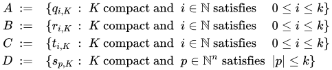



Con esta topología, se convierte en un espacio de Fréchet localmente convexo que no es normable . Cada elemento de es una seminorma continua en Bajo esta topología, una red en converge a si y solo si para cada multiíndice con y cada compacto la red de derivadas parciales converge uniformemente a en [3] Para cualquier subconjunto acotado (von Neumann) de es un subconjunto relativamente compacto de [4] En particular, un subconjunto de está acotado si y solo si está acotado en para todo [4] El espacio es un espacio de Montel si y solo si [5]






Un subconjunto de está abierto en esta topología si y sólo si existe tal que está abierto cuando está dotado de la topología de subespacio inducida en él por


Topología endoa(K)
Como antes, arregle Recuerde que si es cualquier subconjunto compacto de entonces

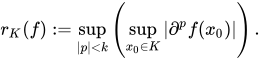
Si es finito entonces es un espacio de Banach [6] con una topología que puede definirse por la norma Y cuando entonces es par un espacio de Hilbert [6] .

Extensiones triviales e independencia dedoa(K) de la topologíatú
Supongamos que es un subconjunto abierto de y es un subconjunto compacto. Por definición, los elementos de son funciones con dominio (en símbolos, ), por lo que el espacio y su topología dependen de para dejar clara esta dependencia del conjunto abierto , denotemos temporalmente por Es importante destacar que, al cambiar el conjunto a un subconjunto abierto diferente (con ) cambiará el conjunto de a [nota 3] de modo que los elementos de serán funciones con dominio en lugar de A pesar de depender del conjunto abierto ( ), la notación estándar para no lo menciona. Esto se justifica porque, como se explicará ahora en esta subsección, el espacio se identifica canónicamente como un subespacio de (tanto algebraica como topológicamente).




Es suficiente explicar cómo identificar canónicamente con cuando uno de y es un subconjunto del otro. La razón es que si y son subconjuntos abiertos arbitrarios de que contienen entonces el conjunto abierto también contiene de modo que cada uno de y se identifica canónicamente con y ahora por transitividad, se identifica por lo tanto con Así que supongamos que son subconjuntos abiertos de que contienen


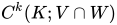


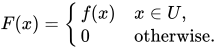
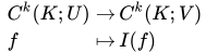
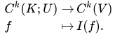
Dada su extensión trivial a es la función definida por: Esta extensión trivial pertenece a (porque tiene soporte compacto) y se denotará por (es decir, ). La asignación induce entonces una función que envía una función en a su extensión trivial en Esta función es una inyección lineal y para cada subconjunto compacto (donde es también un subconjunto compacto de ya que ), Si está restringida a entonces la siguiente función lineal inducida es un homeomorfismo (los homeomorfismos lineales se denominan isomorfismos TVS ): y por lo tanto la siguiente función es una incrustación topológica : Usando la inyección, el espacio vectorial se identifica canónicamente con su imagen en Porque a través de esta identificación, también puede considerarse como un subconjunto de Por lo tanto, la topología en es independiente del subconjunto abierto de que contiene [7] lo que justifica la práctica de escribir en lugar de












Topología LF canónica
Recordemos que denota todas las funciones en que tienen soporte compacto en donde note que es la unión de todos como rangos sobre todos los subconjuntos compactos de Además, para cada uno es un subconjunto denso de El caso especial cuando nos da el espacio de funciones de prueba.


La topología LF canónica no es metrizable y, lo que es más importante, es estrictamente más fina que la topología de subespacio que induce en Sin embargo, la topología LF canónica se convierte en un espacio de Mackey en barril bornológico nuclear [8] de Montel [9] reflexivo completo ; lo mismo es cierto de su espacio dual fuerte (es decir, el espacio de todas las distribuciones con su topología habitual). La topología LF canónica se puede definir de varias maneras.

Distribuciones
Como se discutió anteriormente, las funcionales lineales continuas en a se conocen como distribuciones en Otras definiciones equivalentes se describen a continuación.
Existe un emparejamiento de dualidad canónica entre una distribución y una función de prueba que se denota mediante corchetes angulares por


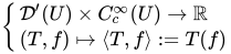
Se interpreta esta notación como la distribución que actúa sobre la función de prueba para dar un escalar, o simétricamente como la función de prueba que actúa sobre la distribución.

Caracterizaciones de distribuciones
Proposición. Si es una función lineal en entonces las siguientes son equivalentes:
- T es una distribución;
- T es continua ;
- T es continua en el origen;
- T es uniformemente continua ;
- T es un operador acotado ;
- T es secuencialmente continua ;
- explícitamente, para cada secuencia en que converge en algún [nota 4]
- T es secuencialmente continua en el origen; en otras palabras, T asigna secuencias nulas [nota 5] a secuencias nulas;
- explícitamente, para cada secuencia en que converge al origen (tal secuencia se llama secuencia nula ),
- Una secuencia nula es por definición cualquier secuencia que converge al origen;
- T asigna secuencias nulas a subconjuntos acotados;
- explícitamente, para cada secuencia que converge al origen, la secuencia está acotada;
- T mapea las secuencias nulas convergentes de Mackey a subconjuntos acotados;
- explícitamente, para cada secuencia nula convergente de Mackey, la secuencia está acotada;
- Se dice que una secuencia es convergente de Mackey al origen si existe una secuencia divergente de números reales positivos tal que la secuencia está acotada; toda secuencia que es convergente de Mackey al origen necesariamente converge al origen (en el sentido habitual);
- El núcleo de T es un subespacio cerrado de
- La gráfica de T es cerrada;
- Existe una seminorma continua tal que
- Existe una constante y un subconjunto finito (donde es cualquier colección de seminormas continuas que define la topología LF canónica en ) tales que [nota 6]
- Para cada subconjunto compacto existen constantes y tales que para todo [1]
- Para cada subconjunto compacto existen constantes y tales que para todos con soporte contenido en [10]
- Para cualquier subconjunto compacto y cualquier secuencia en si converge uniformemente a cero para todos los multiíndices entonces


















Topología en el espacio de distribuciones y su relación con la topología débil-*
El conjunto de todas las distribuciones en es el espacio dual continuo de , que cuando está dotado de la topología dual fuerte se denota por Es importante destacar que, a menos que se indique lo contrario, la topología en es la topología dual fuerte ; si la topología es, en cambio, la topología débil-* , se indicará así. Ninguna topología es metrizable, aunque a diferencia de la topología débil-*, la topología dual fuerte se convierte en un espacio nuclear completo , por nombrar solo algunas de sus propiedades deseables.

Ni su dual fuerte ni su dualidad fuerte son espacios secuenciales y, por lo tanto, ninguna de sus topologías puede describirse completamente mediante secuencias (en otras palabras, definir solo qué secuencias convergen en estos espacios no es suficiente para definir completa/correctamente sus topologías). Sin embargo, una secuencia en converge en la topología dual fuerte si y solo si converge en la topología débil-* (esto lleva a muchos autores a usar la convergencia puntual para definir la convergencia de una secuencia de distribuciones; esto está bien para las secuencias, pero no se garantiza que se extienda a la convergencia de redes de distribuciones porque una red puede converger puntualmente pero no converger en la topología dual fuerte). Se puede encontrar más información sobre la topología con la que está dotada en el artículo sobre espacios de funciones de prueba y distribuciones y en los artículos sobre topologías polares y sistemas duales .
Una función lineal de en otro espacio vectorial topológico localmente convexo (como cualquier espacio normado ) es continua si y solo si es secuencialmente continua en el origen. Sin embargo, esto ya no está garantizado si la función no es lineal o para funciones que tienen valores en espacios topológicos más generales (por ejemplo, que no sean también espacios vectoriales topológicos localmente convexos ). Lo mismo es cierto para las funciones de (de manera más general, esto es cierto para las funciones de cualquier espacio bornológico localmente convexo ).
Localización de distribuciones
No hay forma de definir el valor de una distribución en un punto particular de U . Sin embargo, como es el caso con las funciones, las distribuciones en U se restringen para dar distribuciones en subconjuntos abiertos de U . Además, las distribuciones se determinan localmente en el sentido de que una distribución en todo U se puede ensamblar a partir de una distribución en una cubierta abierta de U que satisface algunas condiciones de compatibilidad en las superposiciones. Tal estructura se conoce como haz .
Extensiones y restricciones a un subconjunto abierto
Sean subconjuntos abiertos de Toda función puede extenderse por cero desde su dominio V a una función en U fijándola igual a en el complemento Esta extensión es una función suave y compacta llamada extensión trivial de a y se denotará por Esta asignación define el operador de extensión trivial que es una función lineal inyectiva continua. Se utiliza para identificar canónicamente como un subespacio vectorial de (aunque no como un subespacio topológico ). Su transpuesta (explicada aquí) se llama restricción a de distribuciones en [11]y como sugiere el nombre, la imagende una distribuciónbajo este mapa es una distribución enllamadarestricción deaLa condición definitoria de la restricciónes: Sientonces el mapa de extensión trivial (lineal inyectivo continuo)noesuna incrustación topológica (en otras palabras, si esta inyección lineal se usara para identificarcomo un subconjunto deentoncesla topología de seríaestrictamente más finaque latopología del subespacioqueinduce en él; lo que es importante,nosería unsubespacio topológicoya que eso requiere igualdad de topologías) y su rango tampoco esdensoen sucodominio[11]En consecuencia, sientonces el mapa de restricción no es ni inyectivo ni sobreyectivo.[11]una distribuciónesextensible a U si pertenece al rango de la transpuesta dey se llamaextensiblesi es extensible a[11]


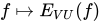








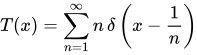
A menos que la restricción a V no sea ni inyectiva ni sobreyectiva . La falta de sobreyectividad se deduce de ello, ya que las distribuciones pueden expandirse hacia el límite de V. Por ejemplo, si y entonces la distribución está en pero no admite extensión a



Pegados y distribuciones que desaparecen en un conjunto
Teorema [12] — Sea una colección de subconjuntos abiertos de Para cada sea y supongamos que para todos la restricción de a es igual a la restricción de a (nótese que ambas restricciones son elementos de ). Entonces existe un único tal que para todos la restricción de T a es igual a





Sea V un subconjunto abierto de U. se dice que se desvanece en V si para todos tales que tenemos T se desvanece en V si y solo si la restricción de T a V es igual a 0, o equivalentemente, si y solo si T se encuentra en el núcleo de la función de restricción.

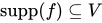


Corolario [12] — Sea una colección de subconjuntos abiertos de y sea si y solo si para cada una la restricción de T a es igual a 0.


Corolario [12] — La unión de todos los subconjuntos abiertos de U en los que una distribución T se desvanece es un subconjunto abierto de U en el que T se desvanece.
Soporte de una distribución
Este último corolario implica que para cada distribución T en U , existe un único subconjunto máximo V de U tal que T se anula en V (y no se anula en ningún subconjunto abierto de U que no esté contenido en V ) ; el complemento en U de este único subconjunto máximo abierto se llama soporte de T . [12] Por lo tanto

Si es una función localmente integrable en U y si es su distribución asociada, entonces el soporte de es el subconjunto cerrado más pequeño de U en cuyo complemento es casi en todas partes igual a 0. [12] Si es continua, entonces el soporte de es igual a la clausura del conjunto de puntos en U en el que no se anula. [12] El soporte de la distribución asociada con la medida de Dirac en un punto es el conjunto [12] Si el soporte de una función de prueba no interseca el soporte de una distribución T entonces Una distribución T es 0 si y solo si su soporte está vacío. Si es idénticamente 1 en algún conjunto abierto que contenga el soporte de una distribución T entonces Si el soporte de una distribución T es compacto entonces tiene orden finito y hay una constante y un entero no negativo tales que: [7]



Si T tiene soporte compacto, entonces tiene una extensión única a una funcional lineal continua en ; esta función puede definirse por donde es cualquier función que sea idénticamente 1 en un conjunto abierto que contenga el soporte de T . [7]

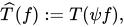

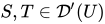
Si y entonces y Por lo tanto, las distribuciones con soporte en un subconjunto dado forman un subespacio vectorial de [13] Además, si es un operador diferencial en U , entonces para todas las distribuciones T en U y todas tenemos y [13]







Distribuciones con soporte compacto
Apoyo en un conjunto de puntos y medidas de Dirac
Para cualquier sea la distribución inducida por la medida de Dirac en Para cualquier distribución y el soporte de T está contenido en si y sólo si T es una combinación lineal finita de derivadas de la medida de Dirac en [14] Si además el orden de T es entonces existen constantes tales que: [15]


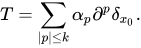
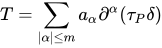
Dicho de otra manera, si T tiene soporte en un único punto , entonces T es de hecho una combinación lineal finita de derivadas distribucionales de la función en P. Es decir, existe un entero m y constantes complejas tales que donde es el operador de traslación.



Distribución con soporte compacto
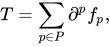
Teorema [7] — Supóngase que T es una distribución en U con soporte compacto K . Existe una función continua definida en U y un multiíndice p tal que donde las derivadas se entienden en el sentido de distribuciones. Es decir, para todas las funciones de prueba en U ,



Distribuciones de orden finito con soporte en un subconjunto abierto
Teorema [7] — Supóngase que T es una distribución en U con soporte compacto K y sea V un subconjunto abierto de U que contiene a K . Puesto que toda distribución con soporte compacto tiene orden finito, tomemos N como el orden de T y definamos Existe una familia de funciones continuas definidas en U con soporte en V tales que donde las derivadas se entienden en el sentido de distribuciones. Es decir, para todas las funciones de prueba en U ,



Estructura global de distribuciones
La definición formal de distribuciones las muestra como un subespacio de un espacio muy grande, a saber, el dual topológico de (o el espacio de Schwartz para distribuciones templadas). La definición no deja claro de inmediato cuán exótica puede ser una distribución. Para responder a esta pregunta, es instructivo ver distribuciones construidas a partir de un espacio más pequeño, a saber, el espacio de funciones continuas. En términos generales, cualquier distribución es localmente una derivada (múltiple) de una función continua. Una versión precisa de este resultado, que se da a continuación, se aplica a distribuciones de soporte compacto, distribuciones templadas y distribuciones generales. En términos generales, ningún subconjunto propio del espacio de distribuciones contiene todas las funciones continuas y está cerrado bajo diferenciación. Esto dice que las distribuciones no son objetos particularmente exóticos; son tan complicadas como sea necesario.

Distribuciones comogavillas
Teorema [16] — Sea T una distribución en U . Existe una secuencia en tal que cada T i tiene soporte compacto y cada subconjunto compacto interseca el soporte de solo un número finito y la secuencia de sumas parciales definida por converge en en T ; en otras palabras, tenemos: Recordemos que una secuencia converge en (con su topología dual fuerte) si y solo si converge puntualmente.




Descomposición de distribuciones como sumas de derivadas de funciones continuas
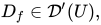
Combinando los resultados anteriores, se puede expresar cualquier distribución en U como la suma de una serie de distribuciones con soporte compacto, donde cada una de estas distribuciones puede a su vez escribirse como una suma finita de derivadas distribucionales de funciones continuas en U. En otras palabras, para arbitrario podemos escribir: donde son conjuntos finitos de multiíndices y las funciones son continuas.
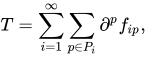


Teorema [17] — Sea T una distribución en U . Para cada p multiíndice existe una función continua en U tal que

- cualquier subconjunto compacto K de U interseca el soporte de sólo un número finito de y

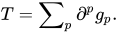
Además, si T tiene orden finito, entonces uno puede elegir de tal manera que sólo un número finito de ellos sean distintos de cero.
Nótese que la suma infinita anterior está bien definida como una distribución. El valor de T para un determinado número puede calcularse utilizando el número finito de que intersecan el soporte de


Operaciones sobre distribuciones
Muchas operaciones que se definen en funciones suaves con soporte compacto también se pueden definir para distribuciones. En general, si es una función lineal que es continua con respecto a la topología débil , entonces no siempre es posible extenderla a una función mediante teoremas de extensión clásicos de topología o análisis funcional lineal. [nota 7] La extensión “distribucional” del operador lineal continuo A anterior es posible si y solo si A admite un adjunto de Schwartz, es decir, otro operador lineal continuo B del mismo tipo tal que , para cada par de funciones de prueba. En esa condición, B es único y la extensión A' es la transpuesta del adjunto de Schwartz B. [ cita requerida ] [18] [ aclaración necesaria ]



Preliminares: Transposición de un operador lineal
Las operaciones sobre distribuciones y espacios de distribuciones se definen a menudo utilizando la transpuesta de un operador lineal. Esto se debe a que la transpuesta permite una presentación unificada de las muchas definiciones en la teoría de distribuciones y también porque sus propiedades son bien conocidas en el análisis funcional . [19] Por ejemplo, el adjunto hermítico bien conocido de un operador lineal entre espacios de Hilbert es simplemente la transpuesta del operador (pero con el teorema de representación de Riesz utilizado para identificar cada espacio de Hilbert con su espacio dual continuo ). En general, la transpuesta de una función lineal continua es la función lineal o, equivalentemente, es la única función que satisface para todos y cada uno (el símbolo primo en no denota una derivada de ningún tipo; simplemente indica que es un elemento del espacio dual continuo ). Dado que es continua, la transpuesta también es continua cuando ambos duales están dotados de sus respectivas topologías duales fuertes ; también es continua cuando ambos duales están dotados de sus respectivas topologías débiles* (consulte los artículos topología polar y sistema dual para obtener más detalles).





En el contexto de las distribuciones, la caracterización de la transpuesta se puede refinar ligeramente. Sea una función lineal continua. Entonces, por definición, la transpuesta de es el único operador lineal que satisface:


Dado que es denso en (aquí, en realidad se refiere al conjunto de distribuciones ), es suficiente que la igualdad definitoria se cumpla para todas las distribuciones de la forma donde Explícitamente, esto significa que una función lineal continua es igual a si y solo si se cumple la condición siguiente: donde el lado derecho es igual a







Operadores diferenciales
Diferenciación de distribuciones
Sea el operador de derivada parcial. Para extender calculamos su transpuesta:

![{\displaystyle {\begin{aligned}\langle {}^{t}A(D_{\psi }),\phi \rangle &=\int _{U}\psi (A\phi )\,dx&&{\text{(Ver arriba.)}}\\&=\int _{U}\psi {\frac {\partial \phi }{\partial x_{k}}}\,dx\\[4pt]&=-\int _{U}\phi {\frac {\partial \psi }{\partial x_{k}}}\,dx&&{\text{(integración por partes)}}\\[4pt]&=-\left\langle {\frac {\partial \psi }{\partial x_{k}}},\phi \right\rangle \\[4pt]&=-\langle A\psi ,\phi \rangle =\langle -A\psi ,\phi \rangle \end{alineado}}}](https://wikimedia.org/api/rest_v1/media/math/render/svg/4af67b152655a622c5db42626dbb10d93d3e9247)
Por lo tanto, la derivada parcial de con respecto a la coordenada se define por la fórmula



Con esta definición, cada distribución es infinitamente diferenciable y la derivada en la dirección es un operador lineal en
De manera más general, si es un multiíndice arbitrario , entonces la derivada parcial de la distribución se define por


La diferenciación de distribuciones es un operador continuo; esta es una propiedad importante y deseable que no comparten la mayoría de las otras nociones de diferenciación.

Si es una distribución en entonces donde es la derivada de y es una traducción por por lo tanto la derivada de puede verse como un límite de cocientes. [20]



Operadores diferenciales que actúan sobre funciones suaves
Un operador diferencial lineal en con coeficientes suaves actúa sobre el espacio de funciones suaves en Dado tal operador, nos gustaría definir una función lineal continua, que extiende la acción de en a distribuciones en En otras palabras, nos gustaría definir tal que el siguiente diagrama conmuta : donde las funciones verticales se dan asignando su distribución canónica que se define por: Con esta notación, la conmutación del diagrama es equivalente a:


![{\displaystyle {\begin{matrix}{\mathcal {D}}'(U)&{\stackrel {D_{P}}{\longrightarrow }}&{\mathcal {D}}'(U)\\[2pt]\uparrow &&\uparrow \\[2pt]C^{\infty }(U)&{\stackrel {P}{\longrightarrow }}&C^{\infty }(U)\end{matrix}}}](https://wikimedia.org/api/rest_v1/media/math/render/svg/97027c86b8d6a85b092e7f318bd7445d2314438b)


Para hallar la transpuesta de la función inducida continua definida por se considera en el lema siguiente. Esto conduce a la siguiente definición del operador diferencial en llamado la transpuesta formal de la cual se denotará por para evitar confusiones con la función transpuesta, que se define por






Lema — Sea un operador diferencial lineal con coeficientes suaves en Entonces para todo tenemos que es equivalente a:



El Lema combinado con el hecho de que la transpuesta formal de la transpuesta formal es el operador diferencial original, es decir, [21] nos permite llegar a la definición correcta: la transpuesta formal induce al operador lineal canónico (continuo) definido por Afirmamos que la transpuesta de esta función, puede tomarse como Para ver esto, para cada calcule su acción sobre una distribución de la forma con :






Llamamos operador lineal continuo al operador diferencial en distribuciones que extienden . [21] Su acción sobre una distribución arbitraria se define mediante:



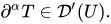
Si converge a entonces para cada multiíndice converge a

Multiplicación de distribuciones por funciones suaves
Un operador diferencial de orden 0 es simplemente la multiplicación por una función suavizada. Y a la inversa, si es una función suavizada entonces es un operador diferencial de orden 0, cuya transpuesta formal es ella misma (es decir, ). El operador diferencial inducido asigna una distribución a una distribución denotada por Hemos definido así la multiplicación de una distribución por una función suavizada.



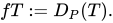
Ahora damos una presentación alternativa de la multiplicación de una distribución en por una función suave. El producto está definido por



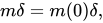
Esta definición coincide con la definición de transposición ya que si es el operador de multiplicación por la función (es decir, ), entonces para que





En la multiplicación por funciones suavizadas, es un módulo sobre el anillo Con esta definición de multiplicación por una función suavizada, la regla del producto ordinaria del cálculo sigue siendo válida. Sin embargo, también surgen algunas identidades inusuales. Por ejemplo, si es la distribución delta de Dirac en entonces y si es la derivada de la distribución delta, entonces




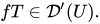
El mapa de multiplicación bilineal dado por no es continuo; sin embargo, es hipocontinuo . [22]


Ejemplo. El producto de cualquier distribución con la función que es idénticamente 1 en es igual a
Ejemplo. Supongamos que es una secuencia de funciones de prueba en que converge a la función constante Para cualquier distribución en la secuencia converge a [23]


Si converge a y converge a entonces converge a

Problema de multiplicación de distribuciones
Es fácil definir el producto de una distribución con una función suave, o más generalmente el producto de dos distribuciones cuyos soportes singulares son disjuntos. [24] Con más esfuerzo, es posible definir un producto de buen comportamiento de varias distribuciones siempre que sus conjuntos de frentes de onda en cada punto sean compatibles. Una limitación de la teoría de distribuciones (y de hiperfunciones) es que no existe un producto asociativo de dos distribuciones que extienda el producto de una distribución por una función suave, como lo demostró Laurent Schwartz en la década de 1950. Por ejemplo, si es la distribución obtenida por el valor principal de Cauchy


Si es la distribución delta de Dirac, entonces pero, por lo que el producto de una distribución por una función suave (que siempre está bien definida) no puede extenderse a un producto asociativo en el espacio de distribuciones.
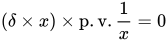
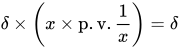
Por lo tanto, los problemas no lineales no se pueden plantear en general y, por lo tanto, no se resuelven solo con la teoría de la distribución. Sin embargo, en el contexto de la teoría cuántica de campos , se pueden encontrar soluciones. En más de dos dimensiones del espacio-tiempo, el problema está relacionado con la regularización de las divergencias . Aquí Henri Epstein y Vladimir Glaser desarrollaron la teoría de perturbación causal matemáticamente rigurosa (pero extremadamente técnica) . Esto no resuelve el problema en otras situaciones. Muchas otras teorías interesantes son no lineales, como por ejemplo las ecuaciones de Navier-Stokes de dinámica de fluidos .
Se han desarrollado varias teorías no enteramente satisfactorias [ cita requerida ] de álgebras de funciones generalizadas , entre las cuales el álgebra (simplificada) de Colombeau es quizás la más popular en uso hoy en día.
Inspired by Lyons' rough path theory,[25] Martin Hairer proposed a consistent way of multiplying distributions with certain structures (regularity structures[26]), available in many examples from stochastic analysis, notably stochastic partial differential equations. See also Gubinelli–Imkeller–Perkowski (2015) for a related development based on Bony's paraproduct from Fourier analysis.
Composition with a smooth function
Let be a distribution on Let be an open set in and If is a submersion then it is possible to define



This is the composition of the distribution with , and is also called the pullback of along , sometimes written

The pullback is often denoted although this notation should not be confused with the use of '*' to denote the adjoint of a linear mapping.

The condition that be a submersion is equivalent to the requirement that the Jacobian derivative of is a surjective linear map for every A necessary (but not sufficient) condition for extending to distributions is that be an open mapping.[27] The Inverse function theorem ensures that a submersion satisfies this condition.


If is a submersion, then is defined on distributions by finding the transpose map. The uniqueness of this extension is guaranteed since is a continuous linear operator on Existence, however, requires using the change of variables formula, the inverse function theorem (locally), and a partition of unity argument.[28]
In the special case when is a diffeomorphism from an open subset of onto an open subset of change of variables under the integral gives:

In this particular case, then, is defined by the transpose formula:

Convolution
Under some circumstances, it is possible to define the convolution of a function with a distribution, or even the convolution of two distributions. Recall that if and are functions on then we denote by the convolution of and defined at to be the integral provided that the integral exists. If are such that then for any functions and we have and [29] If and are continuous functions on at least one of which has compact support, then and if then the value of on do not depend on the values of outside of the Minkowski sum [29]












Importantly, if has compact support then for any the convolution map is continuous when considered as the map or as the map [29]




Translation and symmetry
Given the translation operator sends to defined by This can be extended by the transpose to distributions in the following way: given a distribution the translation of by is the distribution defined by [30][31]








Given define the function by Given a distribution let be the distribution defined by The operator is called the symmetry with respect to the origin.[30]



Convolution of a test function with a distribution
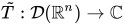
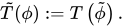
Convolution with defines a linear map: which is continuous with respect to the canonical LF space topology on

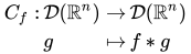

Convolution of with a distribution can be defined by taking the transpose of relative to the duality pairing of with the space of distributions.[32] If then by Fubini's theorem




Extending by continuity, the convolution of with a distribution is defined by

An alternative way to define the convolution of a test function and a distribution is to use the translation operator The convolution of the compactly supported function and the distribution is then the function defined for each by


It can be shown that the convolution of a smooth, compactly supported function and a distribution is a smooth function. If the distribution has compact support, and if is a polynomial (resp. an exponential function, an analytic function, the restriction of an entire analytic function on to the restriction of an entire function of exponential type in to ), then the same is true of [30] If the distribution has compact support as well, then is a compactly supported function, and the Titchmarsh convolution theorem Hörmander (1983, Theorem 4.3.3) implies that: where denotes the convex hull and denotes the support.





Convolution of a smooth function with a distribution
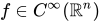
Let and and assume that at least one of and has compact support. The convolution of and denoted by or by is the smooth function:[30] satisfying for all :

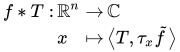

![{\displaystyle {\begin{aligned}&\operatorname {supp} (f\ast T)\subseteq \operatorname {supp} (f)+\operatorname {supp} (T)\\[6pt]&{\text{ for all }}p\in \mathbb {N} ^{n}:\quad {\begin{cases}\partial ^{p}\left\langle T,\tau _{x}{\tilde {f}}\right\rangle =\left\langle T,\partial ^{p}\tau _{x}{\tilde {f}}\right\rangle \\\partial ^{p}(T\ast f)=(\partial ^{p}T)\ast f=T\ast (\partial ^{p}f).\end{cases}}\end{aligned}}}](https://wikimedia.org/api/rest_v1/media/math/render/svg/607c94c3cb33ab03262e95db308c9ecd64a42502)
Let be the map . If is a distribution, then is continuous as a map . If also has compact support, then is also continuous as the map and continuous as the map [30]





If is a continuous linear map such that for all and all then there exists a distribution such that for all [7]




Example.[7] Let be the Heaviside function on For any


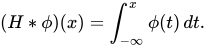
Let be the Dirac measure at 0 and let be its derivative as a distribution. Then and Importantly, the associative law fails to hold:



Convolution of distributions
It is also possible to define the convolution of two distributions and on provided one of them has compact support. Informally, to define where has compact support, the idea is to extend the definition of the convolution to a linear operation on distributions so that the associativity formula continues to hold for all test functions [33]




It is also possible to provide a more explicit characterization of the convolution of distributions.[32] Suppose that and are distributions and that has compact support. Then the linear maps are continuous. The transposes of these maps: are consequently continuous and it can also be shown that[30]



This common value is called the convolution of and and it is a distribution that is denoted by or It satisfies [30] If and are two distributions, at least one of which has compact support, then for any [30] If is a distribution in and if is a Dirac measure then ;[30] thus is the identity element of the convolution operation. Moreover, if is a function then where now the associativity of convolution implies that for all functions and





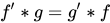

Suppose that it is that has compact support. For consider the function

It can be readily shown that this defines a smooth function of which moreover has compact support. The convolution of and is defined by


This generalizes the classical notion of convolution of functions and is compatible with differentiation in the following sense: for every multi-index


The convolution of a finite number of distributions, all of which (except possibly one) have compact support, is associative.[30]
This definition of convolution remains valid under less restrictive assumptions about and [34]
The convolution of distributions with compact support induces a continuous bilinear map defined by where denotes the space of distributions with compact support.[22] However, the convolution map as a function is not continuous[22] although it is separately continuous.[35] The convolution maps and given by both fail to be continuous.[22] Each of these non-continuous maps is, however, separately continuous and hypocontinuous.[22]
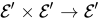






Convolution versus multiplication
In general, regularity is required for multiplication products, and locality is required for convolution products. It is expressed in the following extension of the Convolution Theorem which guarantees the existence of both convolution and multiplication products. Let be a rapidly decreasing tempered distribution or, equivalently, be an ordinary (slowly growing, smooth) function within the space of tempered distributions and let be the normalized (unitary, ordinary frequency) Fourier transform.[36] Then, according to Schwartz (1951), hold within the space of tempered distributions.[37][38][39] In particular, these equations become the Poisson Summation Formula if is the Dirac Comb.[40] The space of all rapidly decreasing tempered distributions is also called the space of convolution operators and the space of all ordinary functions within the space of tempered distributions is also called the space of multiplication operators More generally, and [41][42] A particular case is the Paley-Wiener-Schwartz Theorem which states that and This is because and In other words, compactly supported tempered distributions belong to the space of convolution operators and Paley-Wiener functions better known as bandlimited functions, belong to the space of multiplication operators [43]





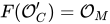
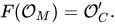
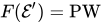
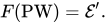


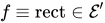
For example, let be the Dirac comb and be the Dirac delta;then is the function that is constantly one and both equations yield the Dirac-comb identity. Another example is to let be the Dirac comb and be the rectangular function; then is the sinc function and both equations yield the Classical Sampling Theorem for suitable functions. More generally, if is the Dirac comb and is a smooth window function (Schwartz function), for example, the Gaussian, then is another smooth window function (Schwartz function). They are known as mollifiers, especially in partial differential equations theory, or as regularizers in physics because they allow turning generalized functions into regular functions.







Tensor products of distributions
Let and be open sets. Assume all vector spaces to be over the field where or For define for every and every the following functions:


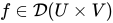



Given and define the following functions: where and These definitions associate every and with the (respective) continuous linear map:








Moreover, if either (resp. ) has compact support then it also induces a continuous linear map of (resp. ).[44]


Fubini's theorem for distributions[44] — Let and If then


The tensor product of and denoted by or is the distribution in defined by:[44]



Spaces of distributions
For all and all every one of the following canonical injections is continuous and has an image (also called the range) that is a dense subset of its codomain: where the topologies on () are defined as direct limits of the spaces in a manner analogous to how the topologies on were defined (so in particular, they are not the usual norm topologies). The range of each of the maps above (and of any composition of the maps above) is dense in its codomain.[45]





Suppose that is one of the spaces (for ) or (for ) or (for ). Because the canonical injection is a continuous injection whose image is dense in the codomain, this map's transpose is a continuous injection. This injective transpose map thus allows the continuous dual space of to be identified with a certain vector subspace of the space of all distributions (specifically, it is identified with the image of this transpose map). This transpose map is continuous but it is not necessarily a topological embedding. A linear subspace of carrying a locally convex topology that is finer than the subspace topology induced on it by is called a space of distributions.[46] Almost all of the spaces of distributions mentioned in this article arise in this way (for example, tempered distribution, restrictions, distributions of order some integer, distributions induced by a positive Radon measure, distributions induced by an -function, etc.) and any representation theorem about the continuous dual space of may, through the transpose be transferred directly to elements of the space












Radon measures
The inclusion map is a continuous injection whose image is dense in its codomain, so the transpose is also a continuous injection.


Note that the continuous dual space can be identified as the space of Radon measures, where there is a one-to-one correspondence between the continuous linear functionals and integral with respect to a Radon measure; that is,

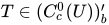
- if then there exists a Radon measure on U such that for all and
- if is a Radon measure on U then the linear functional on defined by sending to is continuous.



Through the injection every Radon measure becomes a distribution on U. If is a locally integrable function on U then the distribution is a Radon measure; so Radon measures form a large and important space of distributions.


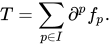
The following is the theorem of the structure of distributions of Radon measures, which shows that every Radon measure can be written as a sum of derivatives of locally functions on U:

Theorem.[47] — Suppose is a Radon measure, where let be a neighborhood of the support of and let There exists a family of locally functions on U such that for every and Furthermore, is also equal to a finite sum of derivatives of continuous functions on where each derivative has order





Positive Radon measures
A linear function on a space of functions is called positive if whenever a function that belongs to the domain of is non-negative (that is, is real-valued and ) then One may show that every positive linear functional on is necessarily continuous (that is, necessarily a Radon measure).[48] Lebesgue measure is an example of a positive Radon measure.


Locally integrable functions as distributions
One particularly important class of Radon measures are those that are induced locally integrable functions. The function is called locally integrable if it is Lebesgue integrable over every compact subset K of U. This is a large class of functions that includes all continuous functions and all Lp space functions. The topology on is defined in such a fashion that any locally integrable function yields a continuous linear functional on – that is, an element of – denoted here by whose value on the test function is given by the Lebesgue integral:


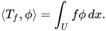
Conventionally, one abuses notation by identifying with provided no confusion can arise, and thus the pairing between and is often written


If and are two locally integrable functions, then the associated distributions and are equal to the same element of if and only if and are equal almost everywhere (see, for instance, Hörmander (1983, Theorem 1.2.5)). Similarly, every Radon measure on defines an element of whose value on the test function is As above, it is conventional to abuse notation and write the pairing between a Radon measure and a test function as Conversely, as shown in a theorem by Schwartz (similar to the Riesz representation theorem), every distribution which is non-negative on non-negative functions is of this form for some (positive) Radon measure.


Test functions as distributions
The test functions are themselves locally integrable, and so define distributions. The space of test functions is sequentially dense in with respect to the strong topology on [49] This means that for any there is a sequence of test functions, that converges to (in its strong dual topology) when considered as a sequence of distributions. Or equivalently,


Distributions with compact support
The inclusion map is a continuous injection whose image is dense in its codomain, so the transpose map is also a continuous injection. Thus the image of the transpose, denoted by forms a space of distributions.[13]



The elements of can be identified as the space of distributions with compact support.[13] Explicitly, if is a distribution on U then the following are equivalent,

- The support of is compact.
- The restriction of to when that space is equipped with the subspace topology inherited from (a coarser topology than the canonical LF topology), is continuous.[13]
- There is a compact subset K of U such that for every test function whose support is completely outside of K, we have


Compactly supported distributions define continuous linear functionals on the space ; recall that the topology on is defined such that a sequence of test functions converges to 0 if and only if all derivatives of converge uniformly to 0 on every compact subset of U. Conversely, it can be shown that every continuous linear functional on this space defines a distribution of compact support. Thus compactly supported distributions can be identified with those distributions that can be extended from to

Distributions of finite order
Let The inclusion map is a continuous injection whose image is dense in its codomain, so the transpose is also a continuous injection. Consequently, the image of denoted by forms a space of distributions. The elements of are the distributions of order [16] The distributions of order which are also called distributions of order 0 are exactly the distributions that are Radon measures (described above).





For a distribution of order k is a distribution of order that is not a distribution of order .[16]


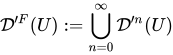
A distribution is said to be of finite order if there is some integer such that it is a distribution of order and the set of distributions of finite order is denoted by Note that if then so that is a vector subspace of , and furthermore, if and only if [16]




Structure of distributions of finite order
Every distribution with compact support in U is a distribution of finite order.[16] Indeed, every distribution in U is locally a distribution of finite order, in the following sense:[16] If V is an open and relatively compact subset of U and if is the restriction mapping from U to V, then the image of under is contained in


The following is the theorem of the structure of distributions of finite order, which shows that every distribution of finite order can be written as a sum of derivatives of Radon measures:
Theorem[16] — Suppose has finite order and Given any open subset V of U containing the support of there is a family of Radon measures in U, such that for very and



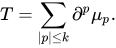
Example. (Distributions of infinite order) Let and for every test function let

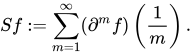
Then is a distribution of infinite order on U. Moreover, can not be extended to a distribution on ; that is, there exists no distribution on such that the restriction of to U is equal to [50]

Tempered distributions and Fourier transform
Defined below are the tempered distributions, which form a subspace of the space of distributions on This is a proper subspace: while every tempered distribution is a distribution and an element of the converse is not true. Tempered distributions are useful if one studies the Fourier transform since all tempered distributions have a Fourier transform, which is not true for an arbitrary distribution in


Schwartz space
The Schwartz space is the space of all smooth functions that are rapidly decreasing at infinity along with all partial derivatives. Thus is in the Schwartz space provided that any derivative of multiplied with any power of converges to 0 as These functions form a complete TVS with a suitably defined family of seminorms. More precisely, for any multi-indices and define



Then is in the Schwartz space if all the values satisfy
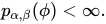
The family of seminorms defines a locally convex topology on the Schwartz space. For the seminorms are, in fact, norms on the Schwartz space. One can also use the following family of seminorms to define the topology:[51]



Otherwise, one can define a norm on via

The Schwartz space is a Fréchet space (that is, a complete metrizable locally convex space). Because the Fourier transform changes into multiplication by and vice versa, this symmetry implies that the Fourier transform of a Schwartz function is also a Schwartz function.


A sequence in converges to 0 in if and only if the functions converge to 0 uniformly in the whole of which implies that such a sequence must converge to zero in [51]



is dense in The subset of all analytic Schwartz functions is dense in as well.[52]

The Schwartz space is nuclear, and the tensor product of two maps induces a canonical surjective TVS-isomorphisms where represents the completion of the injective tensor product (which in this case is identical to the completion of the projective tensor product).[53]


Tempered distributions
The inclusion map is a continuous injection whose image is dense in its codomain, so the transpose is also a continuous injection. Thus, the image of the transpose map, denoted by forms a space of distributions.



The space is called the space of tempered distributions. It is the continuous dual space of the Schwartz space. Equivalently, a distribution is a tempered distribution if and only if


The derivative of a tempered distribution is again a tempered distribution. Tempered distributions generalize the bounded (or slow-growing) locally integrable functions; all distributions with compact support and all square-integrable functions are tempered distributions. More generally, all functions that are products of polynomials with elements of Lp space for are tempered distributions.


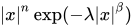
The tempered distributions can also be characterized as slowly growing, meaning that each derivative of grows at most as fast as some polynomial. This characterization is dual to the rapidly falling behaviour of the derivatives of a function in the Schwartz space, where each derivative of decays faster than every inverse power of An example of a rapidly falling function is for any positive


Fourier transform
To study the Fourier transform, it is best to consider complex-valued test functions and complex-linear distributions. The ordinary continuous Fourier transform is a TVS-automorphism of the Schwartz space, and the Fourier transform is defined to be its transpose which (abusing notation) will again be denoted by So the Fourier transform of the tempered distribution is defined by for every Schwartz function is thus again a tempered distribution. The Fourier transform is a TVS isomorphism from the space of tempered distributions onto itself. This operation is compatible with differentiation in the sense that and also with convolution: if is a tempered distribution and is a slowly increasing smooth function on is again a tempered distribution and is the convolution of and In particular, the Fourier transform of the constant function equal to 1 is the distribution.








Expressing tempered distributions as sums of derivatives
If is a tempered distribution, then there exists a constant and positive integers and such that for all Schwartz functions



This estimate, along with some techniques from functional analysis, can be used to show that there is a continuous slowly increasing function and a multi-index such that

Restriction of distributions to compact sets
If then for any compact set there exists a continuous function compactly supported in (possibly on a larger set than K itself) and a multi-index such that on


Using holomorphic functions as test functions
The success of the theory led to an investigation of the idea of hyperfunction, in which spaces of holomorphic functions are used as test functions. A refined theory has been developed, in particular Mikio Sato's algebraic analysis, using sheaf theory and several complex variables. This extends the range of symbolic methods that can be made into rigorous mathematics, for example, Feynman integrals.
See also
- Cauchy principal value – Method for assigning values to certain improper integrals which would otherwise be undefined
- Gelfand triple – Construction linking the study of "bound" and continuous eigenvalues in functional analysisPages displaying short descriptions of redirect targets
- Gelfand–Shilov space
- Generalized function – Objects extending the notion of functions
- Hilbert transform – Integral transform and linear operator
- Homogeneous distribution
- Laplacian of the indicator – Limit of sequence of smooth functions
- Limit of distributions
- Mollifier – Integration kernels for smoothing out sharp features
- Vague topology
Differential equations related
- Fundamental solution – Concept in the solution of linear partial differential equations
- Pseudo-differential operator – Type of differential operator
- Weak solution – Mathematical solution
Generalizations of distributions
- Colombeau algebra – commutative associative differential algebra of generalized functions into which smooth functions (but not arbitrary continuous ones) embed as a subalgebra and distributions embed as a subspacePages displaying wikidata descriptions as a fallback
- Current (mathematics) – Distributions on spaces of differential forms
- Distribution (number theory) – function on finite sets which is analogous to an integralPages displaying wikidata descriptions as a fallback
- Distribution on a linear algebraic group – Linear function satisfying a support condition
- Green's function – Impulse response of an inhomogeneous linear differential operator
- Hyperfunction – Type of generalized function
- Malgrange–Ehrenpreis theorem
Notes
- ^ Note that being an integer implies This is sometimes expressed as Since the inequality "" means: if while if then it means
- ^ The image of the compact set under a continuous -valued map (for example, for ) is itself a compact, and thus bounded, subset of If then this implies that each of the functions defined above is -valued (that is, none of the supremums above are ever equal to ).
- ^ Exactly as with the space is defined to be the vector subspace of consisting of maps with support contained in endowed with the subspace topology it inherits from .
- ^ Even though the topology of is not metrizable, a linear functional on is continuous if and only if it is sequentially continuous.
- ^ A null sequence is a sequence that converges to the origin.
- ^ If is also directed under the usual function comparison then we can take the finite collection to consist of a single element.
- ^ The extension theorem for mappings defined from a subspace S of a topological vector space E to the topological space E itself works for non-linear mappings as well, provided they are assumed to be uniformly continuous. But, unfortunately, this is not our case, we would desire to “extend” a linear continuous mapping A from a tvs E into another tvs F, in order to obtain a linear continuous mapping from the dual E’ to the dual F’ (note the order of spaces). In general, this is not even an extension problem, because (in general) E is not necessarily a subset of its own dual E’. Moreover, It is not a classic topological transpose problem, because the transpose of A goes from F’ to E’ and not from E’ to F’. Our case needs, indeed, a new order of ideas, involving the specific topological properties of the Laurent Schwartz spaces D(U) and D’(U), together with the fundamental concept of weak (or Schwartz) adjoint of the linear continuous operator A.
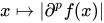
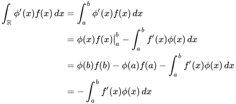
- ^ For example, let and take to be the ordinary derivative for functions of one real variable and assume the support of to be contained in the finite interval then since where the last equality is because










References
- ^ a b Trèves 2006, pp. 222–223.
- ^ Grubb 2009, p. 14
- ^ Trèves 2006, pp. 85–89.
- ^ a b Trèves 2006, pp. 142–149.
- ^ Trèves 2006, pp. 356–358.
- ^ a b Trèves 2006, pp. 131–134.
- ^ a b c d e f g Rudin 1991, pp. 149–181.
- ^ Trèves 2006, pp. 526–534.
- ^ Trèves 2006, p. 357.
- ^ See for example Grubb 2009, p. 14.
- ^ a b c d Trèves 2006, pp. 245–247.
- ^ a b c d e f g Trèves 2006, pp. 253–255.
- ^ a b c d e Trèves 2006, pp. 255–257.
- ^ Trèves 2006, pp. 264–266.
- ^ Rudin 1991, p. 165.
- ^ a b c d e f g Trèves 2006, pp. 258–264.
- ^ Rudin 1991, pp. 169–170.
- ^ Strichartz, Robert (1993). A Guide to Distribution Theory and Fourier Transforms. USA. p. 17.
{{cite book}}: CS1 maint: location missing publisher (link) - ^ Strichartz 1994, §2.3; Trèves 2006.
- ^ Rudin 1991, p. 180.
- ^ a b Trèves 2006, pp. 247–252.
- ^ a b c d e Trèves 2006, p. 423.
- ^ Trèves 2006, p. 261.
- ^ Per Persson (username: md2perpe) (Jun 27, 2017). "Multiplication of two distributions whose singular supports are disjoint". Stack Exchange Network.
{{cite web}}: CS1 maint: numeric names: authors list (link) - ^ Lyons, T. (1998). "Differential equations driven by rough signals". Revista Matemática Iberoamericana. 14 (2): 215–310. doi:10.4171/RMI/240.
- ^ Hairer, Martin (2014). "A theory of regularity structures". Inventiones Mathematicae. 198 (2): 269–504. arXiv:1303.5113. Bibcode:2014InMat.198..269H. doi:10.1007/s00222-014-0505-4. S2CID 119138901.
- ^ See for example Hörmander 1983, Theorem 6.1.1.
- ^ See Hörmander 1983, Theorem 6.1.2.
- ^ a b c Trèves 2006, pp. 278–283.
- ^ a b c d e f g h i j Trèves 2006, pp. 284–297.
- ^ See for example Rudin 1991, §6.29.
- ^ a b Trèves 2006, Chapter 27.
- ^ Hörmander 1983, §IV.2 proves the uniqueness of such an extension.
- ^ See for instance Gel'fand & Shilov 1966–1968, v. 1, pp. 103–104 and Benedetto 1997, Definition 2.5.8.
- ^ Trèves 2006, p. 294.
- ^ Folland, G.B. (1989). Harmonic Analysis in Phase Space. Princeton, NJ: Princeton University Press.
- ^ Horváth, John (1966). Topological Vector Spaces and Distributions. Reading, MA: Addison-Wesley Publishing Company.
- ^ Barros-Neto, José (1973). An Introduction to the Theory of Distributions. New York, NY: Dekker.
- ^ Petersen, Bent E. (1983). Introduction to the Fourier Transform and Pseudo-Differential Operators. Boston, MA: Pitman Publishing.
- ^ Woodward, P.M. (1953). Probability and Information Theory with Applications to Radar. Oxford, UK: Pergamon Press.
- ^ Trèves 2006, pp. 318–319.
- ^ Friedlander, F.G.; Joshi, M.S. (1998). Introduction to the Theory of Distributions. Cambridge, UK: Cambridge University Press.
- ^ Schwartz 1951.
- ^ a b c Trèves 2006, pp. 416–419.
- ^ Trèves 2006, pp. 150–160.
- ^ Trèves 2006, pp. 240–252.
- ^ Trèves 2006, pp. 262–264.
- ^ Trèves 2006, p. 218.
- ^ Trèves 2006, pp. 300–304.
- ^ Rudin 1991, pp. 177–181.
- ^ a b Trèves 2006, pp. 92–94.
- ^ Trèves 2006, p. 160.
- ^ Trèves 2006, p. 531.
Bibliography
- Barros-Neto, José (1973). An Introduction to the Theory of Distributions. New York, NY: Dekker.
- Benedetto, J.J. (1997), Harmonic Analysis and Applications, CRC Press.
- Folland, G.B. (1989). Harmonic Analysis in Phase Space. Princeton, NJ: Princeton University Press.
- Friedlander, F.G.; Joshi, M.S. (1998). Introduction to the Theory of Distributions. Cambridge, UK: Cambridge University Press..
- Gårding, L. (1997), Some Points of Analysis and their History, American Mathematical Society.
- Gel'fand, I.M.; Shilov, G.E. (1966–1968), Generalized functions, vol. 1–5, Academic Press.
- Grubb, G. (2009), Distributions and Operators, Springer.
- Hörmander, L. (1983), The analysis of linear partial differential operators I, Grundl. Math. Wissenschaft., vol. 256, Springer, doi:10.1007/978-3-642-96750-4, ISBN 3-540-12104-8, MR 0717035.
- Horváth, John (1966). Topological Vector Spaces and Distributions. Addison-Wesley series in mathematics. Vol. 1. Reading, MA: Addison-Wesley Publishing Company. ISBN 978-0201029857.
- Kolmogorov, Andrey; Fomin, Sergei V. (1957). Elements of the Theory of Functions and Functional Analysis. Dover Books on Mathematics. New York: Dover Books. ISBN 978-1-61427-304-2. OCLC 912495626.
- Narici, Lawrence; Beckenstein, Edward (2011). Topological Vector Spaces. Pure and applied mathematics (Second ed.). Boca Raton, FL: CRC Press. ISBN 978-1584888666. OCLC 144216834.
- Petersen, Bent E. (1983). Introduction to the Fourier Transform and Pseudo-Differential Operators. Boston, MA: Pitman Publishing..
- Rudin, Walter (1991). Functional Analysis. International Series in Pure and Applied Mathematics. Vol. 8 (Second ed.). New York, NY: McGraw-Hill Science/Engineering/Math. ISBN 978-0-07-054236-5. OCLC 21163277.
- Schaefer, Helmut H.; Wolff, Manfred P. (1999). Topological Vector Spaces. GTM. Vol. 8 (Second ed.). New York, NY: Springer New York Imprint Springer. ISBN 978-1-4612-7155-0. OCLC 840278135.
- Schwartz, Laurent (1954), "Sur l'impossibilité de la multiplications des distributions", C. R. Acad. Sci. Paris, 239: 847–848.
- Schwartz, Laurent (1951), Théorie des distributions, vol. 1–2, Hermann.
- Sobolev, S.L. (1936), "Méthode nouvelle à résoudre le problème de Cauchy pour les équations linéaires hyperboliques normales", Mat. Sbornik, 1: 39–72.
- Stein, Elias; Weiss, Guido (1971), Introduction to Fourier Analysis on Euclidean Spaces, Princeton University Press, ISBN 0-691-08078-X.
- Strichartz, R. (1994), A Guide to Distribution Theory and Fourier Transforms, CRC Press, ISBN 0-8493-8273-4.
- Trèves, François (2006) [1967]. Topological Vector Spaces, Distributions and Kernels. Mineola, N.Y.: Dover Publications. ISBN 978-0-486-45352-1. OCLC 853623322.
- Woodward, P.M. (1953). Probability and Information Theory with Applications to Radar. Oxford, UK: Pergamon Press.
Further reading
- M. J. Lighthill (1959). Introduction to Fourier Analysis and Generalised Functions. Cambridge University Press. ISBN 0-521-09128-4 (requires very little knowledge of analysis; defines distributions as limits of sequences of functions under integrals)
- V.S. Vladimirov (2002). Methods of the theory of generalized functions. Taylor & Francis. ISBN 0-415-27356-0
- Vladimirov, V.S. (2001) [1994], "Generalized function", Encyclopedia of Mathematics, EMS Press.
- Vladimirov, V.S. (2001) [1994], "Generalized functions, space of", Encyclopedia of Mathematics, EMS Press.
- Vladimirov, V.S. (2001) [1994], "Generalized function, derivative of a", Encyclopedia of Mathematics, EMS Press.
- Vladimirov, V.S. (2001) [1994], "Generalized functions, product of", Encyclopedia of Mathematics, EMS Press.
- Oberguggenberger, Michael (2001) [1994], "Generalized function algebras", Encyclopedia of Mathematics, EMS Press.