 Hispanopedia Wiki
En el análisis funcional y áreas relacionadas de las matemáticas , un espacio vectorial topológico completo es un espacio vectorial topológico (TVS) con la propiedad de que siempre que los puntos se acercan progresivamente entre sí, entonces existe algún punto hacia el cual todos se acercan. La noción de "puntos que se acercan progresivamente" se hace rigurosa mediante las redes de Cauchy o filtros de Cauchy , que son generalizaciones de las sucesiones de Cauchy , mientras que "punto hacia el cual todos se acercan" significa que esta red o filtro de Cauchy converge a La noción de completitud para los TVS utiliza la teoría de espacios uniformes como marco para generalizar la noción de completitud para los espacios métricos . Pero a diferencia de la completitud métrica, la completitud de los TVS no depende de ninguna métrica y está definida para todos los TVS, incluidos aquellos que no son metrizables o Hausdorff .


La completitud es una propiedad extremadamente importante que debe poseer un espacio vectorial topológico. Las nociones de completitud para espacios normados y TVS metrizables , que se definen comúnmente en términos de completitud de una norma o métrica particular, se pueden reducir a esta noción de completitud TVS, una noción que es independiente de cualquier norma o métrica particular. Un espacio vectorial topológico metrizable con una métrica invariante de traslación [nota 1] es completo como un TVS si y solo si es un espacio métrico completo , lo que por definición significa que cada secuencia de - Cauchy converge a algún punto en Ejemplos destacados de TVS completos que también son metrizables incluyen todos los espacios F y, en consecuencia, también todos los espacios de Fréchet , espacios de Banach y espacios de Hilbert . Ejemplos destacados de TVS completos que (normalmente) no son metrizables incluyen espacios LF estrictos como el espacio de funciones de prueba con su topología LF canónica, el espacio dual fuerte de cualquier espacio de Fréchet no normalizable , así como muchas otras topologías polares en espacios duales continuos u otras topologías en espacios de mapas lineales .


Explícitamente, un espacio vectorial topológico (TVS) es completo si cada red , o equivalentemente, cada filtro , que es Cauchy con respecto a la uniformidad canónica del espacio necesariamente converge a algún punto. Dicho de otra manera, un TVS es completo si su uniformidad canónica es una uniformidad completa . La uniformidad canónica en un TVS es la única [nota 2] uniformidad invariante en la traducción que induce en la topología Esta noción de "completitud de TVS" depende solo de la resta vectorial y de la topología del TVS; en consecuencia, se puede aplicar a todos los TVS, incluidos aquellos cuyas topologías no se pueden definir en términos de métricas o pseudometrías . Un TVS de primer orden contable es completo si y solo si cada secuencia de Cauchy (o equivalentemente, cada filtro de Cauchy elemental ) converge a algún punto.


Todo espacio vectorial topológico, incluso si no es metrizable o no es Hausdorff , tiene una completitud , que por definición es un TVS completo en el que se puede incorporar un TVS como un subespacio vectorial denso . Además, cada TVS de Hausdorff tiene una completitud de Hausdorff , que es necesariamente única hasta el isomorfismo TVS . Sin embargo, como se analiza a continuación, todos los TVS tienen infinitas completitudes no Hausdorff que no son isomorfas entre sí.


Definiciones
En esta sección se resume la definición de un espacio vectorial topológico (TVS) completo en términos de redes y prefiltros . Se puede encontrar información sobre la convergencia de redes y filtros, como definiciones y propiedades, en el artículo sobre filtros en topología .
Cada espacio vectorial topológico (TVS) es un grupo topológico conmutativo con identidad bajo la adición y la uniformidad canónica de un TVS se define enteramente en términos de resta (y por lo tanto de adición); no interviene la multiplicación escalar y no se necesita ninguna estructura adicional.
Uniformidad canónica
La diagonal de es el conjunto [1] y para cualquier séquito canónico /vecindad alrededores el conjunto donde sientoncescontiene la diagonal



![{\displaystyle {\begin{alignedat}{4}\Delta _{X}(N)~&~{\stackrel {\scriptscriptstyle {\text{def}}}{=}}~\{(x,y)\en X\times X~:~xy\en N\}=\bigcup _{y\en X}[(y+N)\times \{y\}]\\&=\Delta _{X}+(N\times \{0\})\end{alignedat}}}](https://wikimedia.org/api/rest_v1/media/math/render/svg/df0a0b869a5222827ffebbcfbd07d4506ca44310)



Si es un conjunto simétrico (es decir, si ), entonces es simétrico , lo que por definición significa que se cumple donde y además, la composición de este conjunto simétrico consigo mismo es:



![{\displaystyle {\begin{alignedat}{4}\Delta _{X}(N)\circ \Delta _{X}(N)~&~{\stackrel {\scriptscriptstyle {\text{def}}}{=}}~\left\{(x,z)\en X\times X~:~{\text{ existe }}y\en X{\text{ tal que }}x,z\en y+N\right\}=\bigcup _{y\en X}[(y+N)\times (y+N)]\\&=\Delta _{X}+(N\times N).\end{alignedat}}}](https://wikimedia.org/api/rest_v1/media/math/render/svg/08cf32daec2444340c56e4ebc82cdf2f898dc728)
Si es cualquier base de vecindad en el origen en entonces la familia de subconjuntos de es un prefiltro en Si es el filtro de vecindad en el origen en entonces forma una base de séquitos para una estructura uniforme en que se considera canónica. [2] Explícitamente, por definición, la La uniformidad canónica inducidapor [2]es elfiltrogeneradopor el prefiltro anterior: dondedenota elcierre ascendentedeen La misma uniformidad canónica resultaría al utilizar una base de vecindad del origen en lugar del filtro de todas las vecindades del origen. Sies cualquier base de vecindad en el origen enentonces el filtrogenerado por el prefiltroes igual a la uniformidad canónicainducida por








Red de Cauchy
La teoría general de espacios uniformes tiene su propia definición de "prefiltro de Cauchy" y "red de Cauchy". Para la uniformidad canónica de estas definiciones, redúzcalas a las que se dan a continuación.
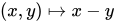
Supongamos que es una red en y es una red en El producto se convierte en un conjunto dirigido al declarar si y solo si y Entonces denota el ( cartesiano )producto neto , donde en particularSientonces la imagen de esta red bajo el mapa de adición vectorialdenota lasuma de estas dos redes:[3] y de manera similar susLa diferencia se define como la imagen del producto neto bajo el mapa de sustracción de vectores: en particular, la notacióndenota lared indexaday no lared indexadaya que usar esta última como definición haría que la notación fuera inútil.


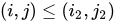










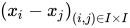


Una red en una TVS se llama red de Cauchy [4] si Explícitamente, esto significa que para cada vecindad de en existe algún índice tal que para todos los índices que satisfacen y es suficiente verificar cualquiera de estas condiciones definitorias para cualquier base de vecindad dada de en Una secuencia de Cauchy es una secuencia que también es una red de Cauchy.



Si entonces en y por lo tanto la continuidad de la función de sustracción vectorial que se define por garantiza que en donde y Esto demuestra que toda red convergente es una red de Cauchy. Por definición, un espacio se llama completo si la recíproca también es siempre cierta. Es decir, es completo si y solo si se cumple lo siguiente:



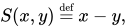



- siempre que una red en entonces converge (a algún punto) en si y solo si en


Una caracterización similar de completitud se mantiene si se utilizan filtros y prefiltros en lugar de redes.
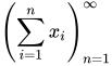
Una serie se llamaSerie de Cauchy (respectivamente, unaserie convergente ) si la secuencia desumas parciales es unasecuencia de Cauchy(respectivamente, unasecuencia convergente).[5]Toda serie convergente es necesariamente una serie de Cauchy. En una TVS completa, toda serie de Cauchy es necesariamente una serie convergente.

Filtro Cauchy y prefiltro Cauchy
Un prefiltro en un espacio vectorial topológico se denomina prefiltro de Cauchy [6] si satisface cualquiera de las siguientes condiciones equivalentes:

- en
- La familia es un prefiltro.
- Explícitamente, significa que para cada vecindad del origen en existen tales que
- en
- La familia es un prefiltro equivalente a ( equivalencia significa que estos prefiltros generan el mismo filtro en ).
- Explícitamente, significa que para cada vecindad del origen en existe alguna tal que
- Porque cada vecindad del origen en contiene algún conjunto -pequeño (es decir, existe alguno tal que ). [6]
- Un subconjunto se llama -pequeño opequeño de orden [6]si
- Para cada vecindad del origen en existe algún y algún tal que [6]
- Esta afirmación sigue siendo verdadera si " " se reemplaza por " "
- Cada vecindad del origen en contiene algún subconjunto de la forma donde y








Es suficiente comprobar cualquiera de las condiciones anteriores para cualquier vecindad dada en Un filtro de Cauchy es un prefiltro de Cauchy que también es un filtro en
Si es un prefiltro en un espacio vectorial topológico y si entonces en si y sólo si y es Cauchy. [3]


Subconjunto completo
Para cualquier prefiltro , es necesariamente un subconjunto de ; es decir,


Un subconjunto de un TVS se denominasubconjunto completo si satisface alguna de las siguientes condiciones equivalentes:
- Cada prefiltro de Cauchy converge al menos a un punto de
- Si es Hausdorff entonces cada prefiltro en convergerá como máximo a un punto de Pero si no es Hausdorff entonces un prefiltro puede converger a múltiples puntos en Lo mismo es cierto para las redes.
- Toda red de Cauchy converge al menos a un punto de
- es un espacio uniforme completo (según la definición de topología de conjuntos de puntos de " espacio uniforme completo ") cuando está dotado de la uniformidad inducida en él por la uniformidad canónica de


El subconjunto se llamasubconjunto secuencialmente completo si cada secuencia de Cauchy en(o equivalentemente, cada filtro/prefiltro de Cauchy elemental en) converge al menos a un punto de
Es importante destacar que la convergencia a puntos fuera de no impide que un conjunto sea completo : si no es Hausdorff y si cada prefiltro de Cauchy en converge a algún punto de entonces será completo incluso si algunos o todos los prefiltros de Cauchy en también convergen a puntos en En resumen, no hay ningún requisito de que estos prefiltros de Cauchy en converjan solo a puntos en Lo mismo puede decirse de la convergencia de las redes de Cauchy en


En consecuencia, si un TVS no es Hausdorff entonces cada subconjunto del cierre de en es completo porque es compacto y cada conjunto compacto es necesariamente completo. En particular, si es un subconjunto propio, como por ejemplo, entonces sería completo aunque cada red de Cauchy en (y también cada prefiltro de Cauchy en ) converja a cada punto en incluyendo aquellos puntos en que no pertenecen a Este ejemplo también muestra que los subconjuntos completos (y de hecho, incluso los subconjuntos compactos) de un TVS no Hausdorff pueden no ser cerrados. Por ejemplo, si entonces si y solo si es cerrado en




Espacio vectorial topológico completo
Un espacio vectorial topológico se denominaespacio vectorial topológico completo si se cumple alguna de las siguientes condiciones equivalentes:
- es un espacio uniforme completo cuando está dotado de su uniformidad canónica.
- En la teoría general de espacios uniformes , un espacio uniforme se denomina espacio uniforme completo si cada filtro de Cauchy en converge a algún punto de en la topología inducida por la uniformidad. Cuando es un TVS, la topología inducida por la uniformidad canónica es igual a la topología dada de (por lo que la convergencia en esta topología inducida es simplemente la convergencia habitual en ).
- es un subconjunto completo de sí mismo.
- Existe un vecindario del origen en que también es un subconjunto completo de [6]
- Esto implica que cada TVS localmente compacto es completo (incluso si el TVS no es Hausdorff).
- Cada prefiltro de Cauchy converge en al menos un punto de
- Si es Hausdorff entonces cada prefiltro en convergerá como máximo a un punto de Pero si no es Hausdorff entonces un prefiltro puede converger a múltiples puntos en Lo mismo es cierto para las redes.
- Cada filtro de Cauchy converge en al menos un punto de
- Toda red de Cauchy converge en al menos un punto de

donde si además es pseudometrizable o metrizable (por ejemplo, un espacio normado ) entonces esta lista puede extenderse para incluir:
- es secuencialmente completo.
Un espacio vectorial topológico escompletar secuencialmente si se cumple alguna de las siguientes condiciones equivalentes:
- es un subconjunto secuencialmente completo de sí mismo.
- Toda secuencia de Cauchy converge en al menos un punto de
- Cada prefiltro de Cauchy elemental converge en al menos un punto de
- Todo filtro de Cauchy elemental converge al menos en un punto de
Unicidad de la uniformidad canónica
La existencia de la uniformidad canónica se demostró anteriormente definiéndola. El teorema que se muestra a continuación establece que la uniformidad canónica de cualquier TVS es la única uniformidad que es (1) invariante en la traducción y (2) genera en la topología.
Teorema [7] (Existencia y unicidad de la uniformidad canónica) — La topología de cualquier TVS puede derivarse de una uniformidad única invariante en la traducción. Si es cualquier base de vecindad del origen, entonces la familia es una base para esta uniformidad.


Esta sección está dedicada a explicar los significados precisos de los términos involucrados en esta declaración de unicidad.
Espacios uniformes y uniformidades invariantes a la traducción
Para cualquier subconjunto sea [1] y sea Una familia no vacía se llama base de séquitos o unasistema fundamental de séquitos sies unprefiltroalsatisfacer todas las condiciones siguientes:




- Todo conjunto en contiene la diagonal de como subconjunto; es decir, para cada Dicho de otra manera, el prefiltro se fija en
- Para cada uno existe algo tal que
- Para cada uno existe algo tal que




Auniformidad oLa estructura uniforme esunfiltroquese genera por alguna base de séquitosen cuyo caso decimos quees unabase de séquitos para


Para un grupo aditivo conmutativo aEl sistema fundamental de entornos invariante en la traducción [7]es un sistema fundamental de entornostal que para cadasi y sólo sipara todauniformidad Ase denomina uniformidad invariante a la traducción [7]si tiene una base de séquitos que es invariante a la traducción. La uniformidad canónica en cualquier TVS es invariante a la traducción.[7]




El operador binario satisface todo lo siguiente:

- Si y entonces
- Asociatividad:
- Identidad:
- Cero:







Séquitos simétricos
Llamemos simétrico a un subconjunto si que es equivalente a Esta equivalencia se sigue de la identidad y del hecho de que si entonces si y sólo si Por ejemplo, el conjunto es siempre simétrico para cada Y porque si y son simétricos entonces también lo es





Topología generada por una uniformidad
Parientes
Sean arbitrarios y sean las proyecciones canónicas sobre las primeras y segundas coordenadas, respectivamente.

Para cualquier definición donde (respectivamente, ) se llama el conjunto de parientes izquierdos (respectivamente, derechos ) de (puntos en) Denote el caso especial donde es un conjunto singleton para algunos por: Si entonces Además, derecho se distribuye tanto sobre uniones como intersecciones, lo que significa que si entonces y












Barrios y espacios abiertos
Dos puntos y son -cercanos si y un subconjunto se llama -pequeño si


Seamos una base de séquitos en Elprefiltro de vecindad en un puntoy, respectivamente, en un subconjuntoson lasfamilias de conjuntos: y los filtrosque cada uno genera se conocen comoFiltro de vecindad de(respectivamente, de). Asignar a cadaprefiltro de vecindad y utilizar ladefinición de vecindad de "conjunto abierto"para obtener unatopologíaenllamadatopología inducida poro latopología inducida . Explícitamente, un subconjuntoes abierto en esta topología si y solo si para cadauno existe algunotal quees decir,es abierto si y solo si para cadauno existe algunotal que






El cierre de un subconjunto en esta topología es:

Prefiltros Cauchy y uniformidades completas
Un prefiltro en un espacio uniforme con uniformidad se llama prefiltro de Cauchy si para cada entorno existe alguno tal que


Un espacio uniforme se llamaespacio uniforme completo (respectivamente, unespacio uniforme secuencialmente completo ) si cada prefiltro de Cauchy (respectivamente, cada prefiltro de Cauchy elemental) enconverge al menos a un punto decuandoestá dotado de la topología inducida por

Caso de un espacio vectorial topológico
Si es un espacio vectorial topológico, entonces para cualquier y y la topología inducida en por la uniformidad canónica es la misma que la topología que comenzó con (es decir, es ).


Continuidad uniforme
Sean y sean TVS, y sea una función. Entonces es uniformemente continua si para cada entorno del origen en existe un entorno del origen en tal que para todo si entonces



Supongamos que es uniformemente continua. Si es una red de Cauchy en entonces es una red de Cauchy en Si es un prefiltro de Cauchy en (lo que significa que es una familia de subconjuntos de que es Cauchy en ) entonces es un prefiltro de Cauchy en Sin embargo, si es un filtro de Cauchy en entonces aunque será un prefiltro de Cauchy , será un filtro de Cauchy en si y solo si es sobreyectiva.



Completitud de TVS vs completitud de (pseudo)métricas
Preliminares: Espacios pseudométricos completos
Repasamos las nociones básicas relacionadas con la teoría general de espacios pseudométricos completos. Recordemos que toda métrica es pseudométrica y que una pseudométrica es una métrica si y solo si implica Por lo tanto, todo espacio métrico es un espacio pseudométrico y un espacio pseudométrico es un espacio métrico si y solo si es una métrica.


Si es un subconjunto de un espacio pseudométrico entonces el diámetro de se define como

Un prefiltro en un espacio pseudométrico se llama prefiltro de Cauchy o simplemente prefiltro de Cauchy si para cada real hay alguno tal que el diámetro de es menor que


Supongamos que es un espacio pseudométrico. Una red en se llama red de Cauchy o simplemente red de Cauchy si es un prefiltro de Cauchy, lo que sucede si y solo si

- para cada hay alguno tal que si con y entonces


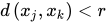
o equivalentemente, si y sólo si en Esto es análogo a la siguiente caracterización de la convergencia de a un punto: si entonces en si y sólo si en


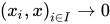
Una secuencia de Cauchy es una secuencia que también es una red de Cauchy. [nota 3]
Toda pseudometría en un conjunto induce la topología canónica usual en la que denotaremos por ; también induce una uniformidad canónica en la que denotaremos por La topología en inducida por la uniformidad es igual a Una red en es de Cauchy con respecto a si y solo si es de Cauchy con respecto a la uniformidad El espacio pseudométrico es un espacio pseudométrico completo (resp. secuencialmente completo) si y solo si es un espacio uniforme completo (resp. secuencialmente completo). Además, el espacio pseudométrico (resp. el espacio uniforme ) es completo si y solo si es secuencialmente completo.


Un espacio pseudométrico (por ejemplo, un espacio métrico ) se denomina completo y se denomina pseudométrico completo si se cumple alguna de las siguientes condiciones equivalentes:
- Cada prefiltro de Cauchy converge al menos a un punto de
- La declaración anterior pero con la palabra "prefiltro" reemplazada por "filtro".
- Toda red de Cauchy converge al menos a un punto de
- Si es una métrica en entonces cualquier punto límite es necesariamente único y lo mismo es cierto para los límites de los prefiltros de Cauchy en
- Toda secuencia de Cauchy en converge al menos a un punto de
- Por lo tanto, para demostrar que es completa, basta considerar únicamente las secuencias de Cauchy (y no es necesario considerar las redes de Cauchy más generales).
- La uniformidad canónica inducida por la pseudometría es una uniformidad completa.
Y si la adición es una métrica, entonces podemos agregar a esta lista:
- Toda secuencia decreciente de bolas cerradas cuyos diámetros se reducen a tiene una intersección no vacía. [8]
Pseudometría completa y TVS completa
Todo espacio F , y por lo tanto también todo espacio de Fréchet , espacio de Banach y espacio de Hilbert es un sistema de sucesión transitoria completo. Nótese que todo espacio F es un espacio de Baire , pero hay espacios normados que son de Baire pero no de Banach. [9]
Se dice que una pseudométrica en un espacio vectorial es unatraducción invariante pseudométrica sipara todos los vectores

Supóngase que es un TVS pseudometrizable (por ejemplo, un TVS metrizable) y que es cualquier pseudométrico en tal que la topología en inducida por es igual a Si es invariante a la traslación, entonces es un TVS completo si y solo si es un espacio pseudométrico completo. [10] Si no es invariante a la traslación, entonces puede ser posible que sea un TVS completo pero no sea un espacio pseudométrico completo [10] (véase esta nota al pie [nota 4] para un ejemplo). [10]
Teorema [11] [12] (Klee) — Sea cualquier [nota 5] métrica en un espacio vectorial tal que la topología inducida por en se convierta en un espacio vectorial topológico. Si es un espacio métrico completo entonces es un TVS completo.
Normas completas y normas equivalentes
Dos normas en un espacio vectorial se denominan equivalentes si y solo si inducen la misma topología. [13] Si y son dos normas equivalentes en un espacio vectorial , entonces el espacio normado es un espacio de Banach si y solo si es un espacio de Banach. Véase esta nota al pie para un ejemplo de una norma continua en un espacio de Banach que no es equivalente a la norma dada de ese espacio de Banach. [nota 6] [13] Todas las normas en un espacio vectorial de dimensión finita son equivalentes y todo espacio normado de dimensión finita es un espacio de Banach. [14] Todo espacio de Banach es un TVS completo. Un espacio normado es un espacio de Banach (es decir, su métrica inducida por la norma canónica es completa) si y solo si es completo como espacio vectorial topológico.


Terminaciones
Una compleción [15] de un TVS es un TVS completo que contiene un subespacio vectorial denso que es TVS-isomorfo a En otras palabras, es un TVS completo en el que se puede realizar una incrustación TVS como un subespacio vectorial denso . Cada incrustación TVS es una incrustación uniforme .
Todo espacio vectorial topológico tiene una completitud. Además, cada TVS de Hausdorff tiene una completitud de Hausdorff , que es necesariamente única hasta el isomorfismo TVS . Sin embargo, todos los TVS, incluso aquellos que son Hausdorff, (ya) completos y/o metrizables tienen infinitas completitudes no Hausdorff que no son isomorfas TVS entre sí.
Ejemplos de finalizaciones
Por ejemplo, el espacio vectorial que consiste en funciones simples de valores escalares para los cuales (donde esta seminorma se define de la manera usual en términos de integración de Lebesgue ) se convierte en un espacio seminorma cuando se le dota de esta seminorma, lo que a su vez lo convierte en un espacio pseudométrico y en un TVS no completo no Hausdorff; cualquier completitud de este espacio es un espacio seminorma completo no Hausdorff que cuando se cociente por la clausura de su origen (para obtener un TVS de Hausdorff ) da como resultado (un espacio linealmente isométrico-isomorfo a) el espacio de Hausdorff completo usual (dotado de la norma completa usual ).


Como otro ejemplo que demuestra la utilidad de las completaciones, las completaciones de productos tensoriales topológicos , como productos tensoriales proyectivos o productos tensoriales inyectivos , del espacio de Banach con un TVS localmente convexo de Hausdorff completo da como resultado un TVS completo que es TVS-isomorfo a un espacio "generalizado" que consiste en funciones -valuadas en (donde este TVS "generalizado" se define de manera análoga al espacio original de funciones escalares en ). De manera similar, la completación del producto tensorial inyectivo del espacio de funciones de prueba -valuadas escalares con dicho TVS es TVS-isomorfo al TVS definido de manera análoga de funciones de prueba -valuadas .


No unicidad de todas las finalizaciones
Como muestra el ejemplo siguiente, independientemente de si un espacio es de Hausdorff o ya completo, cada espacio vectorial topológico (TVS) tiene infinitas completitudes no isomorfas. [16]
Sin embargo, cada TVS de Hausdorff tiene una completitud de Hausdorff que es única hasta el isomorfismo TVS. [16] Pero, no obstante, cada TVS de Hausdorff todavía tiene infinitas completitudes no isomorfas no Hausdorff.
Ejemplo ( No unicidad de las compleciones ): [15] Sea cualquier TVS completo y sea cualquier TVS dotado de la topología indiscreta , que recuerda convierte en un TVS completo. Puesto que tanto y son TVS completos, entonces es su producto Si y son subconjuntos abiertos no vacíos de y respectivamente, entonces y lo que muestra que es un subespacio denso de Por lo tanto, por definición de "compleción", es una compleción de (no importa que ya esté completo). Así que al identificar con si es un subespacio vectorial denso de entonces tiene tanto y como compleciones.





Terminaciones de Hausdorff
Cada TVS de Hausdorff tiene una completitud de Hausdorff que es única hasta el isomorfismo TVS. [16] Pero, sin embargo, como se muestra arriba, cada TVS de Hausdorff todavía tiene infinitas completitudes no isomorfas no Hausdorff.
Propiedades de las terminaciones de Hausdorff [17] — Supóngase que y son TVS de Hausdorff con completación. Supóngase que es una incrustación de TVS en un subespacio vectorial denso de Entonces


- Propiedad universal : para cada función lineal continua en una TVS de Hausdorff completa existe una única función lineal continua tal que


Si es una incrustación TVS en un subespacio vectorial denso de una TVS de Hausdorff completa que tiene la propiedad universal anterior, entonces existe un isomorfismo TVS (biyectivo) único tal que



Corolario [17] — Supongamos que es un TVS de Hausdorff completo y es un subespacio vectorial denso de Entonces, cada mapa lineal continuo en un TVS de Hausdorff completo tiene una extensión lineal continua única a un mapa


Existencia de terminaciones de Hausdorff
Un filtro de Cauchy en un TVS se llamafiltro de Cauchy mínimo [17]sinoexiste un filtro de Cauchy enque sea estrictamente más grueso que(es decir, "estrictamente más grueso que" significa contenido como un subconjunto propio de).
Si es un filtro de Cauchy en entonces el filtro generado por el siguiente prefiltro: es el único filtro de Cauchy mínimo en que está contenido como un subconjunto de [17] En particular, para cualquier filtro de vecindad en es un filtro de Cauchy mínimo.


Sea el conjunto de todos los filtros de Cauchy mínimos en y sea el mapa definido enviando al filtro de vecindad de en Endow con la siguiente estructura de espacio vectorial: Dado y un escalar sea (resp. ) el único filtro de Cauchy mínimo contenido en el filtro generado por (resp. ).



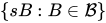
Para cada barrio equilibrado del origen en let

Si es Hausdorff, entonces la colección de todos los conjuntos como rangos sobre todos los vecindarios equilibrados del origen en forma una topología vectorial al convertirse en un TVS de Hausdorff completo. Además, la función es una incrustación de TVS en un subespacio vectorial denso de [17]


Si es un TVS metrizable , entonces se puede construir una compleción de Hausdorff de utilizando clases de equivalencia de secuencias de Cauchy en lugar de filtros de Cauchy mínimos.
Terminaciones no Hausdorff
En esta subsección se detalla cómo cada TVS no Hausdorff puede ser embebido en un subespacio vectorial denso de un TVS completo. La prueba de que cada TVS Hausdorff tiene una completitud Hausdorff está ampliamente disponible y, por lo tanto, este hecho se utilizará (sin prueba) para mostrar que cada TVS no Hausdorff también tiene una completitud. Estos detalles son a veces útiles para extender los resultados de los TVS Hausdorff a los TVS no Hausdorff.
Sea la clausura del origen en donde está dotado de su topología de subespacio inducida por (de modo que tiene la topología indiscreta ). Como tiene la topología trivial, se muestra fácilmente que todo subespacio vectorial de que es un complemento algebraico de en es necesariamente un complemento topológico de en [18] [19] Sea cualquier complemento topológico de en el que es necesariamente un TVS de Hausdorff (ya que es TVS-isomorfo al cociente TVS [nota 7] ). Como es la suma directa topológica de y (lo que significa que en la categoría de TVS), la función canónica es un isomorfismo TVS. [19] Sea la inversa de esta función canónica. (Como nota al margen, se deduce que todo subconjunto abierto y todo subconjunto cerrado de satisface [prueba 1] )





El TVS de Hausdorff puede ser incrustado por TVS, digamos a través del mapa en un subespacio vectorial denso de su completitud . Dado que y son completos, también lo es su producto. Denotemos el mapa identidad y observemos que el mapa producto es una incrustación por TVS cuya imagen es densa en Definamos el mapa [nota 8] que es una incrustación por TVS de en un subespacio vectorial denso del TVS completo. Además, observemos que el cierre del origen en es igual a y que y son complementos topológicos en






Para resumir, [19] dado cualquier complemento algebraico (y por lo tanto topológico) de en y dada cualquier completitud del TVS de Hausdorff tal que entonces la inclusión natural [20] es una incrustación TVS bien definida de en un subespacio vectorial denso del TVS completo donde además,





Topología de una terminación
Teorema [7] [21] (Topología de una completitud) — Sea un TVS completo y sea un subespacio vectorial denso de Si es cualquier vecindad base del origen en entonces el conjunto es una vecindad del origen en la completitud de


Si es localmente convexo y es una familia de seminormas continuas en que generan la topología de entonces la familia de todas las extensiones continuas de de todos los miembros de es una familia generadora de seminormas para

Dicho de otra manera, si es una completitud de un TVS con y si es una base de vecindad del origen en entonces la familia de conjuntos es una base de vecindad en el origen en [3]


Teorema [22] (Completaciones de cocientes) — Sea un espacio vectorial topológico metrizable y sea un subespacio vectorial cerrado de Supóngase que es una completitud de Entonces la completitud de es TVS-isomorfa a Si además es un espacio normado, entonces este TVS-isomorfismo es también una isometría.


Teorema de completitud de Grothendieck
Sea el que denotacompactología equicontinua en el espacio dual continuoque por definición consiste en todoslos subconjuntos absolutamente convexosequicontinuosdébilmente cerradosy débilmenteacotadosde[23](que son necesariamente subconjuntos débilmente compactos de). Supóngase que cadaestá dotado de latopología débilmente compactaSe dice queunfiltroen convergen continuamente asi existe algúncontenedor(es decir,) tal que la traza deenla que es la familiaconverge aen(es decir, sien la topología débil-* dada).[24] El filtroconverge continuamente asi y solo siconverge continuamente al origen, lo que sucede si y solo si para cadafiltroen el campo escalar (que eso) dondedenota cualquier base de vecindad en el origen endenota elemparejamiento de dualidad, ydenota el filtro generado por[24] una funciónen un espacio topológico (comoo) es -continuo si siempre que un filtroconvergecontinuamente aentonces[24]











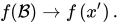
Teorema de completitud de Grothendieck [24] — Sies un espacio vectorial topológico de Hausdorff, entonces su completitud es linealmente isomorfa al conjunto de todas las funciones lineales γ {\displaystyle \gamma } -continuas en

Propiedades preservadas por terminaciones
Si un TVS tiene alguna de las siguientes propiedades, también las tiene su finalización:
- Hausdorff
- Localmente convexo
- Pseudometrizable [16]
- Metrizable [16]
- Semi-normalizable
- Normalizable
- Además, si es un espacio normado, entonces la completitud puede elegirse para que sea un espacio de Banach tal que la incrustación TVS de en sea una isometría.
- Hausdorff pre-Hilbert , es decir, una TVS inducida por un producto interno . [25]
- Nuclear [26]
- Cañón [27]
- Mackey [28]
- Espacio DF [29]

Completaciones de espacios de Hilbert
Todo espacio de producto interno tiene una completitud que es un espacio de Hilbert, donde el producto interno es la única extensión continua a del producto interno original. La norma inducida por es también la única extensión continua a de la norma inducida por [25] [21]


Otras propiedades conservadas
Si es un TVS de Hausdorff , entonces el espacio dual continuo de es idéntico al espacio dual continuo de la compleción de [30] La compleción de un espacio bornológico localmente convexo es un espacio en barril . [27] Si y son DF-espacios , entonces el producto tensorial proyectivo , así como su compleción, de estos espacios es un DF-espacio. [31]
La compleción del producto tensorial proyectivo de dos espacios nucleares es nuclear. [26] La compleción de un espacio nuclear es TVS-isomorfa con un límite proyectivo de espacios de Hilbert . [26]
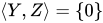
Si (lo que significa que el mapa de adición es un isomorfismo TVS) tiene una completitud de Hausdorff , entonces Si además es un espacio de producto interno y y son complementos ortogonales entre sí en (es decir, ), entonces y son complementos ortogonales en el espacio de Hilbert





Propiedades de los mapas conservados por extensiones a una terminación
Si es un operador lineal nuclear entre dos espacios localmente convexos y si es una completitud de entonces tiene una extensión lineal continua única a un operador lineal nuclear [26]


Sean y dos TVS de Hausdorff con completa. Sea una completitud de Sea el espacio vectorial de operadores lineales continuos y sea la función que envía cada a su única extensión lineal continua en Entonces es un isomorfismo de espacio vectorial (sobreyectivo). Además, asigna familias de subconjuntos equicontinuos entre sí. Supóngase que está dotado de una G {\displaystyle {\mathcal {G}}} -topología y que denota las clausuras en de conjuntos en Entonces la función es también un isomorfismo TVS. [26]





Ejemplos y condiciones suficientes para un TVS completo
Teorema — [11] Sea cualquier métrica (no se supone que sea invariante a la traslación) en un espacio vectorial tal que la topología inducida por en se convierta en un espacio vectorial topológico. Si es un espacio métrico completo, entonces es un TVS completo.
- Cualquier sistema de telemetría de transmisión dotado de la topología trivial es completo y cada uno de sus subconjuntos es completo. Además, todo sistema de telemetría de transmisión con la topología trivial es compacto y, por lo tanto, localmente compacto. Por lo tanto, un sistema de telemetría de transmisión completo, seminormable, localmente convexo y localmente compacto no necesita ser de dimensión finita si no es de Hausdorff.
- Un producto arbitrario de SVT completos (o secuencialmente completos, cuasicompletos) tiene esa misma propiedad. Si todos los espacios son de Hausdorff, entonces las recíprocas también son verdaderas. [32] Un producto de compleciones de Hausdorff de una familia de SVT (de Hausdorff) es una compleción de Hausdorff de su SVT producto. [32] De manera más general, un producto arbitrario de subconjuntos completos de una familia de SVT es un subconjunto completo del SVT producto. [33]
- El límite proyectivo de un sistema proyectivo de sistemas de transición de álgebra completos de Hausdorff (resp. secuencialmente completos, cuasi-completos) tiene esa misma propiedad. [32] Un límite proyectivo de completitud de Hausdorff de un sistema inverso de sistemas de transición de álgebra (de Hausdorff) es una completitud de Hausdorff de su límite proyectivo. [32]
- Si es un subespacio vectorial cerrado de un TVS pseudometrizable completo entonces el espacio cociente es completo. [3]
- Supóngase que es un subespacio vectorial completo de un TVS metrizable. Si el espacio cociente es completo, entonces también lo es [3] [34] Sin embargo, existe un TVS completo que tiene un subespacio vectorial cerrado tal que el TVS cociente no es completo. [17]
- Cada espacio F , espacio de Fréchet , espacio de Banach y espacio de Hilbert es un TVS completo.
- Los espacios LF estrictos y los espacios LB estrictos son completos. [35]
- Supongamos que es un subconjunto denso de un TVS. Si cada filtro de Cauchy en converge a algún punto en entonces es completo. [34]
- El espacio de Schwartz de funciones suaves está completo.
- Los espacios de distribuciones y funciones de prueba están completos.
- Suppose that and are locally convex TVSs and that the space of continuous linear maps is endowed with the topology of uniform convergence on bounded subsets of If is a bornological space and if is complete then is a complete TVS.[35] In particular, the strong dual of a bornological space is complete.[35] However, it need not be bornological.
- Every quasi-complete DF-space is complete.[29]
- Let and be Hausdorff TVS topologies on a vector space such that If there exists a prefilter such that is a neighborhood basis at the origin for and such that every is a complete subset of then is a complete TVS.[6]


Properties
Complete TVSs
Every TVS has a completion and every Hausdorff TVS has a Hausdorff completion.[36] Every complete TVS is quasi-complete space and sequentially complete.[37] However, the converses of the above implications are generally false.[37] There exists a sequentially complete locally convex TVS that is not quasi-complete.[29]
If a TVS has a complete neighborhood of the origin then it is complete.[38] Every complete pseudometrizable TVS is a barrelled space and a Baire space (and thus non-meager).[39] The dimension of a complete metrizable TVS is either finite or uncountable.[19]
Cauchy nets and prefilters
Any neighborhood basis of any point in a TVS is a Cauchy prefilter.
Every convergent net (respectively, prefilter) in a TVS is necessarily a Cauchy net (respectively, a Cauchy prefilter).[6] Any prefilter that is subordinate to (that is, finer than) a Cauchy prefilter is necessarily also a Cauchy prefilter[6] and any prefilter finer than a Cauchy prefilter is also a Cauchy prefilter. The filter associated with a sequence in a TVS is Cauchy if and only if the sequence is a Cauchy sequence. Every convergent prefilter is a Cauchy prefilter.
If is a TVS and if is a cluster point of a Cauchy net (respectively, Cauchy prefilter), then that Cauchy net (respectively, that Cauchy prefilter) converges to in [3] If a Cauchy filter in a TVS has an accumulation point then it converges to
Uniformly continuous maps send Cauchy nets to Cauchy nets.[3] A Cauchy sequence in a Hausdorff TVS when considered as a set, is not necessarily relatively compact (that is, its closure in is not necessarily compact[note 9]) although it is precompact (that is, its closure in the completion of is compact).
Every Cauchy sequence is a bounded subset but this is not necessarily true of Cauchy net. For example, let have it usual order, let denote any preorder on the non-indiscrete TVS (that is, does not have the trivial topology; it is also assumed that ) and extend these two preorders to the union by declaring that holds for every and Let be defined by if and otherwise (that is, if ), which is a net in since the preordered set is directed (this preorder on is also partial order (respectively, a total order) if this is true of ). This net is a Cauchy net in because it converges to the origin, but the set is not a bounded subset of (because does not have the trivial topology).



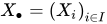
Suppose that is a family of TVSs and that denotes the product of these TVSs. Suppose that for every index is a prefilter on Then the product of this family of prefilters is a Cauchy filter on if and only if each is a Cauchy filter on [17]


Maps
If is an injective topological homomorphism from a complete TVS into a Hausdorff TVS then the image of (that is, ) is a closed subspace of [34] If is a topological homomorphism from a complete metrizable TVS into a Hausdorff TVS then the range of is a closed subspace of [34] If is a uniformly continuous map between two Hausdorff TVSs then the image under of a totally bounded subset of is a totally bounded subset of [40]

Uniformly continuous extensions
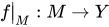
Suppose that is a uniformly continuous map from a dense subset of a TVS into a complete Hausdorff TVS Then has a unique uniformly continuous extension to all of [3] If in addition is a homomorphism then its unique uniformly continuous extension is also a homomorphism.[3] This remains true if "TVS" is replaced by "commutative topological group."[3] The map is not required to be a linear map and that is not required to be a vector subspace of
Uniformly continuous linear extensions
Suppose be a continuous linear operator between two Hausdorff TVSs. If is a dense vector subspace of and if the restriction to is a topological homomorphism then is also a topological homomorphism.[41] So if and are Hausdorff completions of and respectively, and if is a topological homomorphism, then 's unique continuous linear extension is a topological homomorphism. (Note that it's possible for to be surjective but for to not be injective.)[41]


Suppose and are Hausdorff TVSs, is a dense vector subspace of and is a dense vector subspaces of If are and are topologically isomorphic additive subgroups via a topological homomorphism then the same is true of and via the unique uniformly continuous extension of (which is also a homeomorphism).[42]
Subsets
Complete subsets
Every complete subset of a TVS is sequentially complete. A complete subset of a Hausdorff TVS is a closed subset of [3][38]
Every compact subset of a TVS is complete (even if the TVS is not Hausdorff or not complete).[3][38] Closed subsets of a complete TVS are complete; however, if a TVS is not complete then is a closed subset of that is not complete. The empty set is complete subset of every TVS. If is a complete subset of a TVS (the TVS is not necessarily Hausdorff or complete) then any subset of that is closed in is complete.[38]
Topological complements
If is a non-normable Fréchet space on which there exists a continuous norm then contains a closed vector subspace that has no topological complement.[29] If is a complete TVS and is a closed vector subspace of such that is not complete, then does not have a topological complement in [29]
Subsets of completions
Let be a separable locally convex metrizable topological vector space and let be its completion. If is a bounded subset of then there exists a bounded subset of such that [29]


Relation to compact subsets
A subset of a TVS (not assumed to be Hausdorff or complete) is compact if and only if it is complete and totally bounded.[43][proof 2] Thus a closed and totally bounded subset of a complete TVS is compact.[44][3]
In a Hausdorff locally convex TVS, the convex hull of a precompact set is again precompact.[45] Consequently, in a complete locally convex Hausdorff TVS, the closed convex hull of a compact subset is again compact.[46]
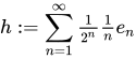
The convex hull of compact subset of a Hilbert space is not necessarily closed and so also not necessarily compact. For example, let be the separable Hilbert space of square-summable sequences with the usual norm and let be the standard orthonormal basis (that is at the -coordinate). The closed set is compact but its convex hull is not a closed set because belongs to the closure of in but (since every sequence is a finite convex combination of elements of and so is necessarily in all but finitely many coordinates, which is not true of ).[47] However, like in all complete Hausdorff locally convex spaces, the closed convex hull of this compact subset is compact.[46] The vector subspace is a pre-Hilbert space when endowed with the substructure that the Hilbert space induces on it but is not complete and (since ). The closed convex hull of in (here, "closed" means with respect to and not to as before) is equal to which is not compact (because it is not a complete subset). This shows that in a Hausdorff locally convex space that is not complete, the closed convex hull of compact subset might fail to be compact (although it will be precompact/totally bounded).









Every complete totally bounded set is relatively compact.[3] If is any TVS then the quotient map is a closed map[48] and thus A subset of a TVS is totally bounded if and only if its image under the canonical quotient map is totally bounded.[19] Thus is totally bounded if and only if is totally bounded. In any TVS, the closure of a totally bounded subset is again totally bounded.[3] In a locally convex space, the convex hull and the disked hull of a totally bounded set is totally bounded.[36] If is a subset of a TVS such that every sequence in has a cluster point in then is totally bounded.[19] A subset of a Hausdorff TVS is totally bounded if and only if every ultrafilter on is Cauchy, which happens if and only if it is pre-compact (that is, its closure in the completion of is compact).[40]



If is compact, then and this set is compact. Thus the closure of a compact set is compact[note 10] (that is, all compact sets are relatively compact).[49] Thus the closure of a compact set is compact. Every relatively compact subset of a Hausdorff TVS is totally bounded.[40]

In a complete locally convex space, the convex hull and the disked hull of a compact set are both compact.[36] More generally, if is a compact subset of a locally convex space, then the convex hull (resp. the disked hull ) is compact if and only if it is complete.[36] Every subset of is compact and thus complete.[proof 3] In particular, if is not Hausdorff then there exist compact complete sets that are not closed.[3]


See also
- Complete metric space – Metric geometry
- Filter (set theory) – Family of sets representing "large" sets
- Filters in topology – Use of filters to describe and characterize all basic topological notions and results.
- Metrizable topological vector space – A topological vector space whose topology can be defined by a metric
- Pseudometric space – Generalization of metric spaces in mathematics
- Quasi-complete space – A topological vector space in which every closed and bounded subset is complete
- Sequentially complete
- Topological group – Group that is a topological space with continuous group action
- Uniform space – Topological space with a notion of uniform properties
Notes
- ^ A metric on a vector space is said to be translation invariant if for all vectors A metric that is induced by a norm is always translation invariant.
- ^ Completeness of normed spaces and metrizable TVSs are defined in terms of norms and metrics. In general, many different norms (for example, equivalent norms) and metrics may be used to determine completeness of such space. This stands in contrast to the uniqueness of this translation-invariant canonical uniformity.
- ^ Every sequence is also a net.
- ^ The normed space is a Banach space where the absolute value is a norm that induces the usual Euclidean topology on Define a metric on by for all where one may show that induces the usual Euclidean topology on However, is not a complete metric since the sequence defined by is a -Cauchy sequence that does not converge in to any point of Note also that this -Cauchy sequence is not a Cauchy sequence in (that is, it is not a Cauchy sequence with respect to the norm ).
- ^ Not assumed to be translation-invariant.
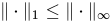
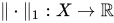
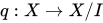
- ^ Let denotes the Banach space of continuous functions with the supremum norm, let where is given the topology induced by and denote the restriction of the L1-norm to by Then one may show that so that the norm is a continuous function. However, is not equivalent to the norm and so in particular, is not a Banach space.
- ^ This particular quotient map is in fact also a closed map.
- ^ Explicitly, this map is defined as follows: for each let and so that Then holds for all and
- ^ If is a normable TVS such that for every Cauchy sequence the closure of in is compact (and thus sequentially compact) then this guarantees that there always exist some such that in Thus any normed space with this property is necessarily sequentially complete. Since not all normed spaces are complete, the closure of a Cauchy sequence is not necessarily compact.
- ^ In general topology, the closure of a compact subset of a non-Hausdorff space may fail to be compact (for example, the particular point topology on an infinite set). This result shows that this does not happen in non-Hausdorff TVSs. The proof uses the fact that is compact (but possibly not closed) and is both closed and compact so that which is the image of the compact set under the continuous addition map is also compact. Recall also that the sum of a compact set (that is, ) and a closed set is closed so is closed in





![{\displaystyle \left(C([0,1]),\|\cdot \|_{\infty }\right)}](https://wikimedia.org/api/rest_v1/media/math/render/svg/a773ac393569c023b8783d3b73fce490446e9022)
![{\displaystyle X=C([0,1])}](https://wikimedia.org/api/rest_v1/media/math/render/svg/5a92f955422c26bcb6edd155506e1168c5f598d0)

![{\displaystyle C([0,1])}](https://wikimedia.org/api/rest_v1/media/math/render/svg/44211c4c325ea7edb9462e7ccecda09841a41216)



![{\displaystyle \left(C([0,1]),\|\cdot \|_{1}\right)}](https://wikimedia.org/api/rest_v1/media/math/render/svg/7dab1443b60234b32432ae500bc320123eff7a50)







Proofs
- ^ Let be a neighborhood of the origin in Since is a neighborhood of in there exists an open (resp. closed) neighborhood of in such that is a neighborhood of the origin. Clearly, is open (resp. closed) if and only if is open (resp. closed). Let so that where is open (resp. closed) if and only if is open (resp. closed).
- ^ Suppose is compact in and let be a Cauchy filter on Let so that is a Cauchy filter of closed sets. Since has the finite intersection property, there exists some such that for all so { (that is, is an accumulation point of ). Since is Cauchy, in Thus is complete. That is also totally bounded follows immediately from the compactness of
- ^ Given any open cover of pick any open set from that cover that contains the origin. Since is a neighborhood of the origin, contains and thus contains









Citations
- ^ a b Schaefer & Wolff 1999, pp. 1–11.
- ^ a b Edwards 1995, p. 61.
- ^ a b c d e f g h i j k l m n o p Narici & Beckenstein 2011, pp. 47–66.
- ^ Narici & Beckenstein 2011, p. 48.
- ^ Zălinescu 2002, pp. 1–23.
- ^ a b c d e f g h Narici & Beckenstein 2011, pp. 48–51.
- ^ a b c d e Schaefer & Wolff 1999, pp. 12–19.
- ^ Narici & Beckenstein 2011, pp. 64–66.
- ^ Wilansky 2013, p. 29.
- ^ a b c Narici & Beckenstein 2011, pp. 47–51.
- ^ a b Schaefer & Wolff 1999, p. 35.
- ^ Klee, V. L. (1952). "Invariant metrics in groups (solution of a problem of Banach)" (PDF). Proc. Amer. Math. Soc. 3 (3): 484–487. doi:10.1090/s0002-9939-1952-0047250-4.
- ^ a b Conrad, Keith. "Equivalence of norms" (PDF). kconrad.math.uconn.edu. Retrieved September 7, 2020.
- ^ see Corollary1.4.18, p.32 in Megginson (1998).
- ^ a b Narici & Beckenstein 2011, pp. 60–61.
- ^ a b c d e Narici & Beckenstein 2011, pp. 93–113.
- ^ a b c d e f g Horváth 1966, pp. 139–141.
- ^ Wilansky 2013, p. 63.
- ^ a b c d e f Schaefer & Wolff 1999, pp. 12–35.
- ^ where for all and
- ^ a b Schaefer & Wolff 1999, pp. 36–72.
- ^ Schaefer & Wolff 1999, pp. 73−121.
- ^ Jarchow 1981, pp. 151, 157.
- ^ a b c d Jarchow 1981, pp. 175−178.
- ^ a b Trèves 2006, pp. 112–125.
- ^ a b c d e Schaefer & Wolff 1999, pp. 73–121.
- ^ a b Schaefer & Wolff 1999, pp. 68–72.
- ^ Schaefer & Wolff 1999, pp. 122–202.
- ^ a b c d e f Schaefer & Wolff 1999, pp. 190–202.
- ^ Narici & Beckenstein 2011, pp. 225–273.
- ^ Schaefer & Wolff 1999, pp. 199–202.
- ^ a b c d Jarchow 1981, pp. 56–73.
- ^ Narici & Beckenstein 2011, p. 57.
- ^ a b c d Horváth 1966, pp. 129–141.
- ^ a b c Narici & Beckenstein 2011, pp. 441–457.
- ^ a b c d Narici & Beckenstein 2011, pp. 67–113.
- ^ a b Narici & Beckenstein 2011, pp. 155–176.
- ^ a b c d Narici & Beckenstein 2011, pp. 115–154.
- ^ Narici & Beckenstein 2011, pp. 371–423.
- ^ a b c Horváth 1966, pp. 145–149.
- ^ a b Schaefer & Wolff 1999, p. 116.
- ^ Narici & Beckenstein 2011, p. 59.
- ^ Narici & Beckenstein 2011, pp. 55–56.
- ^ Narici & Beckenstein 2011, pp. 55–66.
- ^ Trèves 2006, p. 67.
- ^ a b Trèves 2006, p. 145.
- ^ Aliprantis & Border 2006, p. 185.
- ^ Narici & Beckenstein 2011, pp. 107–112.
- ^ Narici & Beckenstein 2011, p. 156.


Bibliography
- Adasch, Norbert; Ernst, Bruno; Keim, Dieter (1978). Topological Vector Spaces: The Theory Without Convexity Conditions. Lecture Notes in Mathematics. Vol. 639. Berlin New York: Springer-Verlag. ISBN 978-3-540-08662-8. OCLC 297140003.
- Aliprantis, Charalambos D.; Border, Kim C. (2006). Infinite Dimensional Analysis: A Hitchhiker's Guide (Third ed.). Berlin: Springer Science & Business Media. ISBN 978-3-540-29587-7. OCLC 262692874.
- Arkhangel'skii, Alexander Vladimirovich; Ponomarev, V.I. (1984). Fundamentals of General Topology: Problems and Exercises. Mathematics and Its Applications. Vol. 13. Dordrecht Boston: D. Reidel. ISBN 978-90-277-1355-1. OCLC 9944489.
- Berberian, Sterling K. (1974). Lectures in Functional Analysis and Operator Theory. Graduate Texts in Mathematics. Vol. 15. New York: Springer. ISBN 978-0-387-90081-0. OCLC 878109401.
- Bogachev, Vladimir I; Smolyanov, Oleg G. (2017). Topological Vector Spaces and Their Applications. Springer Monographs in Mathematics. Cham, Switzerland: Springer International Publishing. ISBN 978-3-319-57117-1. OCLC 987790956.
- Bourbaki, Nicolas (1989) [1966]. General Topology: Chapters 1–4 [Topologie Générale]. Éléments de mathématique. Berlin New York: Springer Science & Business Media. ISBN 978-3-540-64241-1. OCLC 18588129.
- Bourbaki, Nicolas (1987) [1981]. Topological Vector Spaces: Chapters 1–5. Éléments de mathématique. Translated by Eggleston, H.G.; Madan, S. Berlin New York: Springer-Verlag. ISBN 3-540-13627-4. OCLC 17499190.
- Conway, John (1990). A course in functional analysis. Graduate Texts in Mathematics. Vol. 96 (2nd ed.). New York: Springer-Verlag. ISBN 978-0-387-97245-9. OCLC 21195908.
- Dixmier, Jacques (1984). General Topology. Undergraduate Texts in Mathematics. Translated by Berberian, S. K. New York: Springer-Verlag. ISBN 978-0-387-90972-1. OCLC 10277303.
- Dolecki, Szymon; Mynard, Frédéric (2016). Convergence Foundations Of Topology. New Jersey: World Scientific Publishing Company. ISBN 978-981-4571-52-4. OCLC 945169917.
- Dugundji, James (1966). Topology. Boston: Allyn and Bacon. ISBN 978-0-697-06889-7. OCLC 395340485.
- Dunford, Nelson; Schwartz, Jacob T. (1988). Linear Operators. Pure and applied mathematics. Vol. 1. New York: Wiley-Interscience. ISBN 978-0-471-60848-6. OCLC 18412261.
- Edwards, Robert E. (1995). Functional Analysis: Theory and Applications. New York: Dover Publications. ISBN 978-0-486-68143-6. OCLC 30593138.
- Grothendieck, Alexander (1973). Topological Vector Spaces. Translated by Chaljub, Orlando. New York: Gordon and Breach Science Publishers. ISBN 978-0-677-30020-7. OCLC 886098.
- Horváth, John (1966). Topological Vector Spaces and Distributions. Addison-Wesley series in mathematics. Vol. 1. Reading, MA: Addison-Wesley Publishing Company. ISBN 978-0201029857.
- Husain, Taqdir; Khaleelulla, S. M. (1978). Barrelledness in Topological and Ordered Vector Spaces. Lecture Notes in Mathematics. Vol. 692. Berlin, New York, Heidelberg: Springer-Verlag. ISBN 978-3-540-09096-0. OCLC 4493665.
- Jarchow, Hans (1981). Locally convex spaces. Stuttgart: B.G. Teubner. ISBN 978-3-519-02224-4. OCLC 8210342.
- Joshi, K. D. (1983). Introduction to General Topology. New York: John Wiley and Sons Ltd. ISBN 978-0-85226-444-7. OCLC 9218750.
- Khaleelulla, S. M. (1982). Counterexamples in Topological Vector Spaces. Lecture Notes in Mathematics. Vol. 936. Berlin, Heidelberg, New York: Springer-Verlag. ISBN 978-3-540-11565-6. OCLC 8588370.
- Köthe, Gottfried (1983) [1969]. Topological Vector Spaces I. Grundlehren der mathematischen Wissenschaften. Vol. 159. Translated by Garling, D.J.H. New York: Springer Science & Business Media. ISBN 978-3-642-64988-2. MR 0248498. OCLC 840293704.
- Köthe, Gottfried (1979). Topological Vector Spaces II. Grundlehren der mathematischen Wissenschaften. Vol. 237. New York: Springer Science & Business Media. ISBN 978-0-387-90400-9. OCLC 180577972.
- Megginson, Robert E. (1998), An introduction to Banach space theory, Graduate Texts in Mathematics, vol. 183, New York: Springer-Verlag, pp. xx+596, ISBN 0-387-98431-3
- Narici, Lawrence; Beckenstein, Edward (2011). Topological Vector Spaces. Pure and applied mathematics (Second ed.). Boca Raton, FL: CRC Press. ISBN 978-1584888666. OCLC 144216834.
- Osborne, Mason Scott (2013). Locally Convex Spaces. Graduate Texts in Mathematics. Vol. 269. Cham Heidelberg New York Dordrecht London: Springer Science & Business Media. ISBN 978-3-319-02045-7. OCLC 865578438.
- Robertson, Alex P.; Robertson, Wendy J. (1980). Topological Vector Spaces. Cambridge Tracts in Mathematics. Vol. 53. Cambridge England: Cambridge University Press. ISBN 978-0-521-29882-7. OCLC 589250.
- Schaefer, Helmut H.; Wolff, Manfred P. (1999). Topological Vector Spaces. GTM. Vol. 8 (Second ed.). New York, NY: Springer New York Imprint Springer. ISBN 978-1-4612-7155-0. OCLC 840278135.
- Schechter, Eric (1996). Handbook of Analysis and Its Foundations. San Diego, CA: Academic Press. ISBN 978-0-12-622760-4. OCLC 175294365.
- Schubert, Horst (1968). Topology. London: Macdonald & Co. ISBN 978-0-356-02077-8. OCLC 463753.
- Swartz, Charles (1992). An introduction to Functional Analysis. New York: M. Dekker. ISBN 978-0-8247-8643-4. OCLC 24909067.
- Trèves, François (2006) [1967]. Topological Vector Spaces, Distributions and Kernels. Mineola, N.Y.: Dover Publications. ISBN 978-0-486-45352-1. OCLC 853623322.
- Voigt, Jürgen (2020). A Course on Topological Vector Spaces. Compact Textbooks in Mathematics. Cham: Birkhäuser Basel. ISBN 978-3-030-32945-7. OCLC 1145563701.
- Wilansky, Albert (2013). Modern Methods in Topological Vector Spaces. Mineola, New York: Dover Publications, Inc. ISBN 978-0-486-49353-4. OCLC 849801114.
- Willard, Stephen (2004) [1970]. General Topology. Mineola, N.Y.: Dover Publications. ISBN 978-0-486-43479-7. OCLC 115240.
- Zălinescu, Constantin (30 July 2002). Convex Analysis in General Vector Spaces. River Edge, N.J. London: World Scientific Publishing. ISBN 978-981-4488-15-0. MR 1921556. OCLC 285163112 – via Internet Archive.