 Hispanopedia Wiki


En matemáticas , la función W de Lambert , también llamada función omega o producto logarítmico , [1] es una función multivaluada , es decir, las ramas de la relación inversa de la función f ( w ) = we w , donde w es cualquier número complejo y e w es la función exponencial . La función recibe su nombre de Johann Lambert , quien consideró un problema relacionado en 1758. Basándose en el trabajo de Lambert, Leonhard Euler describió la función W per se en 1783.
Para cada entero k hay una rama, denotada por W k ( z ) , que es una función de valor complejo de un argumento complejo. W 0 se conoce como la rama principal . Estas funciones tienen la siguiente propiedad: si z y w son números complejos cualesquiera, entonces

se cumple si y sólo si

Cuando se trata sólo de números reales, las dos ramas W 0 y W −1 son suficientes: para los números reales x e y la ecuación

se puede resolver para y solo si x ≥ − 1/mi ; produce y = W 0 ( x ) si x ≥ 0 y los dos valores y = W 0 ( x ) y y = W −1 ( x ) si − 1/mi ≤ x < 0 .
Las ramas de la función W de Lambert no se pueden expresar en términos de funciones elementales . [2] Es útil en combinatoria , por ejemplo, en la enumeración de árboles . Se puede utilizar para resolver varias ecuaciones que involucran exponenciales (por ejemplo, los máximos de las distribuciones de Planck , Bose–Einstein y Fermi–Dirac ) y también ocurre en la solución de ecuaciones diferenciales de retardo , como y ′( t ) = a y ( t − 1) . En bioquímica , y en particular en cinética enzimática , se describe una solución en forma abierta para el análisis cinético del curso temporal de la cinética de Michaelis–Menten en términos de la función W de Lambert .


Terminología
La convención de notación elegida aquí (con W 0 y W −1 ) sigue la referencia canónica sobre la función W de Lambert de Corless, Gonnet, Hare, Jeffrey y Knuth . [3]
El nombre "logaritmo del producto" se puede entender así: dado que la función inversa de f ( w ) = e w se llama logaritmo , tiene sentido llamar a la "función" inversa del producto we w como "logaritmo del producto". (Nota técnica: al igual que el logaritmo complejo , es multivaluado y, por lo tanto, W se describe como la relación inversa en lugar de la función inversa). Está relacionado con la constante omega , que es igual a W 0 (1) .
Historia
Lambert consideró por primera vez la ecuación trascendental de Lambert relacionada en 1758, [4] lo que condujo a un artículo de Leonhard Euler en 1783 [5] que discutía el caso especial de we w .
La ecuación que Lambert consideró fue

Euler transformó esta ecuación en la forma

Ambos autores derivaron una solución en serie para sus ecuaciones.
Una vez que Euler hubo resuelto esta ecuación, consideró el caso . Tomando límites, derivó la ecuación


Luego puso y obtuvo una solución en serie convergente para la ecuación resultante, expresando en términos de .


Después de tomar derivadas con respecto a y algunas manipulaciones, se obtiene la forma estándar de la función de Lambert.
En 1993, se informó que la función Lambert proporciona una solución exacta al modelo de función delta de Dirac de doble pozo de la mecánica cuántica para cargas iguales [6] , un problema fundamental en física. Impulsados por esto, Rob Corless y los desarrolladores del sistema de álgebra computacional Maple se dieron cuenta de que "la función W de Lambert se ha utilizado ampliamente en muchos campos, pero debido a la notación diferente y la ausencia de un nombre estándar, el conocimiento de la función no era tan alto como debería haber sido". [3] [7]

Otro ejemplo donde se encuentra esta función es en la cinética de Michaelis-Menten . [8]
Aunque se creía ampliamente que la función de Lambert no se puede expresar en términos de funciones elementales ( de Liouvillian ), la primera prueba publicada no apareció hasta 2008. [9]
Propiedades elementales, ramas y rango

_for_various_branches_(n).jpg/1280px-Imaginary_part_of_the_Lambert_W(n,x+i_y)_for_various_branches_(n).jpg)
Hay un número contable de ramas de la función W , denotada por W k ( z ) , para el entero k ; W 0 ( z ) es la rama principal. W 0 ( z ) se define para todos los números complejos z mientras que W k ( z ) con k ≠ 0 se define para todos los z distintos de cero . Con W 0 (0) = 0 ylímitez →0 W k ( z ) = −∞ para todo k ≠ 0 .
El punto de ramificación de la rama principal está en z = − 1/mi , con un corte de rama que se extiende hasta −∞ a lo largo del eje real negativo. Este corte de rama separa la rama principal de las dos ramas W −1 y W 1 . En todas las ramas W k con k ≠ 0 , hay un punto de rama en z = 0 y un corte de rama a lo largo de todo el eje real negativo.
Las funciones W k ( z ), k ∈ Z son todas inyectivas y sus rangos son disjuntos. El rango de toda la función multivaluada W es el plano complejo. La imagen del eje real es la unión del eje real y la cuadratriz de Hipias , la curva paramétrica w = − t cot t + it .
Inverso

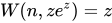


El gráfico de rango anterior también delinea las regiones en el plano complejo donde la simple relación inversa es verdadera. implica que existe un tal que , donde depende del valor de . El valor del entero cambia abruptamente cuando está en el corte de la rama de , lo que significa que ≤ 0 , excepto para donde es ≤ −1/ .





Definiendo , donde y son reales, y expresando en coordenadas polares, se ve que



Para , el corte de rama para es el eje real no positivo, de modo que


y

Para , la rama cortada para es el eje real con , de modo que la desigualdad se convierte en
![{\displaystyle W[n,ze^{z}]}](https://wikimedia.org/api/rest_v1/media/math/render/svg/fb4be5264a023f670dd1e4d4db4fbbffa4b51573)


Dentro de las regiones delimitadas por lo anterior, no hay cambios discontinuos en , y esas regiones especifican dónde la función es simplemente invertible, es decir , .
Cálculo
Derivado
Por diferenciación implícita , se puede demostrar que todas las ramas de W satisfacen la ecuación diferencial

( W no es diferenciable para z = − 1/mi .) Como consecuencia, se obtiene la siguiente fórmula para la derivada de W :

Usando la identidad e W ( z ) = el/W ( z ) , da la siguiente fórmula equivalente:

En el origen tenemos

Integral
La función W ( x ) , y muchas otras expresiones que involucran W ( x ) , se pueden integrar utilizando la sustitución w = W ( x ) , es decir x = we w :
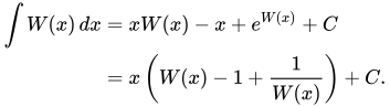
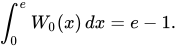
(La última ecuación es más común en la literatura pero no está definida en x = 0 ). Una consecuencia de esto (usando el hecho de que W 0 ( e ) = 1 ) es la identidad
Expansiones asintóticas
La serie de Taylor de W 0 alrededor de 0 se puede encontrar utilizando el teorema de inversión de Lagrange y está dada por

El radio de convergencia es1/mi , como se puede ver mediante la prueba de la razón . La función definida por esta serie se puede extender a una función holomorfa definida en todos los números complejos con un corte de rama a lo largo del intervalo (−∞, − 1/mi ] ; esta función holomorfa define la rama principal de la función W de Lambert .
Para valores grandes de x , W 0 es asintótico a
![{\displaystyle {\begin{aligned}W_{0}(x)&=L_{1}-L_{2}+{\frac {L_{2}}{L_{1}}}+{\frac {L_{2}\left(-2+L_{2}\right)}{2L_{1}^{2}}}+{\frac {L_{2}\left(6-9L_{2}+2L_{2}^{2}\right)}{6L_{1}^{3}}}+{\frac {L_{2}\left(-12+36L_{2}-22L_{2}^{2}+3L_{2}^{3}\right)}{12L_{1}^{4}}}+\cdots \\[5pt]&=L_{1}-L_{2}+\sum _{l=0}^{\infty }\sum _{m=1}^{\infty }{\frac {(-1)^{l}\left[{\begin{smallmatrix}l+m\\l+1\end{smallmatrix}}\right]}{m!}}L_{1}^{-lm}L_{2}^{m},\end{alineado}}}](https://wikimedia.org/api/rest_v1/media/math/render/svg/f5e7cb8d231b7fabe03c2fc5d8845d1c9e18f467)
donde L 1 = ln x , L 2 = ln ln x , y [yo + yo
+ 1] es un número de Stirling no negativodel primer tipo.[3]Manteniendo solo los dos primeros términos de la expansión,

La otra rama real, W −1 , definida en el intervalo [− 1/mi , 0) , tiene una aproximación de la misma forma cuando x tiende a cero, con en este caso L 1 = ln(− x ) y L 2 = ln(−ln(− x )) . [3]
Potencias enteras y complejas
Las potencias enteras de W 0 también admiten expansiones simples en serie de Taylor (o Laurent ) en cero:

De manera más general, para r ∈ Z , la fórmula de inversión de Lagrange da
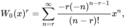
que es, en general, una serie de Laurent de orden r . De manera equivalente, esta última puede escribirse en forma de una expansión de Taylor de potencias de W 0 ( x ) / x :

lo cual es válido para cualquier r ∈ C y | x | < 1/mi .
Límites y desigualdades
Se conocen varios límites no asintóticos para la función de Lambert.
Hoorfar y Hassani [10] demostraron que el siguiente límite se cumple para x ≥ e :

También mostraron el límite general
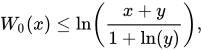
para cada y , con igualdad solo para . El límite permite realizar muchos otros límites, como tomar que da el límite


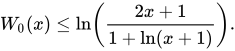
En 2013 se demostró [11] que la rama W −1 se puede acotar de la siguiente manera:

Roberto Iacono y John P. Boyd [12] ampliaron los límites de la siguiente manera:

Identidades

_plotted_in_the_complex_plane_from_-2-2i_to_2+2i.svg/1280px-The_product_logarithm_Lambert_W_function_W_2(z)_plotted_in_the_complex_plane_from_-2-2i_to_2+2i.svg.png)
De la definición se desprenden algunas identidades:

Nótese que, dado que f ( x ) = xe x no es inyectiva , no siempre se cumple que W ( f ( x )) = x , de forma muy similar a lo que ocurre con las funciones trigonométricas inversas . Para x < 0 fijo y x ≠ −1 , la ecuación xe x = ye y tiene dos soluciones reales en y , una de las cuales es, por supuesto, y = x . Entonces, para i = 0 y x < −1 , así como para i = −1 y x ∈ (−1, 0) , y = W i ( xe x ) es la otra solución.
Algunas otras identidades: [13]
- [14]
-
- (que puede extenderse a otros n y x si se elige la rama correcta).
![{\displaystyle {\begin{aligned}&W(x)e^{W(x)}=x,\quad {\text{por lo tanto:}}\\[5pt]&e^{W(x)}={\frac {x}{W(x)}},\qquad e^{-W(x)}={\frac {W(x)}{x}},\qquad e^{nW(x)}=\left({\frac {x}{W(x)}}\right)^{n}.\end{aligned}}}](https://wikimedia.org/api/rest_v1/media/math/render/svg/db7a28b4f31f15aa4730b353d5ef11b206fa43b5)



![{\displaystyle {\begin{aligned}&W(x)=\ln {\frac {x}{W(x)}}&&{\text{para }}x\geq -{\frac {1}{e}},\\[5pt]&W\left({\frac {nx^{n}}{W\left(x\right)^{n-1}}}\right)=nW(x)&&{\text{para }}n,x>0\end{aligned}}}](https://wikimedia.org/api/rest_v1/media/math/render/svg/e834c16fb0e25cf530b84a39bdcc0bba7c75d762)

Sustituyendo −ln x en la definición: [15]
![{\displaystyle {\begin{aligned}W_{0}\left(-{\frac {\ln x}{x}}\right)&=-\ln x&{\text{para }}0&<x\leq e,\\[5pt]W_{-1}\left(-{\frac {\ln x}{x}}\right)&=-\ln x&{\text{para }}x&>e.\end{aligned}}}](https://wikimedia.org/api/rest_v1/media/math/render/svg/108810da107aa426c8708fe1c3eaa34a2da9575e)
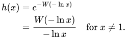
Con la exponencial iterada h ( x ) de Euler :
Valores especiales
Los siguientes son valores especiales de la rama principal:


- (la constante omega )


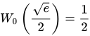
![{\displaystyle W_{0}({\frac {\sqrt[{n}]{e}}{n}}\right)={\frac {1}{n}}}](https://wikimedia.org/api/rest_v1/media/math/render/svg/2a9c8214e48f2f2fb5be14e54203da5d25bb8fb9)

Valores especiales de la rama W −1 :

Representaciones
La rama principal de la función de Lambert se puede representar mediante una integral propia, debida a Poisson: [16]

Kalugin–Jeffrey–Corless encontró otra representación de la rama principal: [17]

La siguiente representación de fracción continua también es válida para la rama principal: [18]
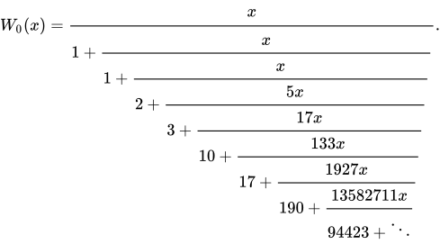
Además, si | W 0 ( x ) | < 1 : [19]
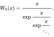
A su vez, si | W 0 ( x ) | > e , entonces
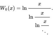
Otras fórmulas
Integrales definidas
Hay varias fórmulas integrales definidas útiles que involucran la rama principal de la función W , incluidas las siguientes:
![{\displaystyle {\begin{aligned}&\int _{0}^{\pi }W_{0}\left(2\cot ^{2}x\right)\sec ^{2}x\,dx=4{\sqrt {\pi }}.\\[5pt]&\int _{0}^{\infty }{\frac {W_{0}(x)}{x{\sqrt {x}}}}\,dx=2{\sqrt {2\pi }}.\\[5pt]&\int _{0}^{\infty }W_{0}\left({\frac {1}{x^{2}}}\right)\,dx={\sqrt {2\pi }}.\end{aligned}}}](https://wikimedia.org/api/rest_v1/media/math/render/svg/e07333d551660a0d3994a68caa2cb780134d6f42)
La primera identidad se puede encontrar escribiendo la integral gaussiana en coordenadas polares .
La segunda identidad se puede derivar haciendo la sustitución u = W 0 ( x ) , lo que da
![{\displaystyle {\begin{aligned}x&=ue^{u},\\[5pt]{\frac {dx}{du}}&=(u+1)e^{u}.\end{aligned}}}](https://wikimedia.org/api/rest_v1/media/math/render/svg/6d9f83a1f16b84fd3408ce93ce89f1165e8c455e)
De este modo
![{\displaystyle {\begin{aligned}\int _{0}^{\infty }{\frac {W_{0}(x)}{x{\sqrt {x}}}}\,dx&=\int _{0}^{\infty }{\frac {u}{ue^{u}{\sqrt {ue^{u}}}}}(u+1)e^{u}\,du\\[5pt]&=\int _{0}^{\infty }{\frac {u+1}{\sqrt {ue^{u}}}}du\\[5pt]&=\int _{0}^{\infty }{\frac {u+1}{\sqrt {u}}}{\frac {1}{\sqrt {e^{u}}}}du\\[5pt]&=\int _{0}^{\infty }u^{\tfrac {1}{2}}e^{-{\frac {u}{2}}}du+\int _{0}^{\infty }u^{-{\tfrac {1}{2}}}e^{-{\frac {u}{2}}}du\\[5pt]&=2\int _{0}^{\infty }(2w)^{\tfrac {1}{2}}e^{-w}\,dw+2\int _{0}^ {\infty }(2w)^{-{\tfrac {1}{2}}}e^{-w}\,dw&&\quad (u=2w)\\[5pt]&=2{\sqrt {2}}\int _ {0}^{\infty }w^{\tfrac {1}{2}}e^{-w}\,dw+{\sqrt {2}}\int _{0}^{\infty }w^{-{\tfrac {1}{2}}}e^{-w}\,dw\\[5pt]&=2{\sqrt {2}}\cdot \Gamma \left({\tfrac {3}{2}}\right)+{\sqrt {2}}\cdot \Gamma \left({\tfrac {1}{2}}\right)\\[5pt]&=2{\sqrt {2}}\left({\tfrac {1}{2}}{\sqrt {\pi }}\right)+{\sqrt {2}}\left({\sqrt {\pi }}\right)\\[5pt]&=2{\sqrt {2\pi }}.\end{alineado}}}](https://wikimedia.org/api/rest_v1/media/math/render/svg/f836d0b33ed568739bf7e32a1ded6e95b08c4429)
La tercera identidad puede derivarse de la segunda haciendo la sustitución u = x −2 y la primera también puede derivarse de la tercera mediante la sustitución z = 1/√ 2 tan x .
A excepción de z a lo largo del corte de la rama (−∞, − 1/mi ] (donde la integral no converge), la rama principal de la función W de Lambert se puede calcular mediante la siguiente integral: [20]
![{\displaystyle {\begin{aligned}W_{0}(z)&={\frac {z}{2\pi }}\int _{-\pi }^{\pi }{\frac {\left( 1-\nu \cot \nu \right)^{2}+\nu ^{2}}{z+\nu \csc \nu e^{-\nu \cot \nu }}}\,d\nu \ \[5pt]&={\frac {z}{\pi }}\int _{0}^{\pi }{\frac {\left(1-\nu \cot \nu \right)^{2} +\nu ^{2}}{z+\nu \csc \nu e^{-\nu \cot \nu }}}\,d\nu ,\end{aligned}}}](https://wikimedia.org/api/rest_v1/media/math/render/svg/fa9c98a56088bb89fee6bf5658dfc3770b289b0c)
donde las dos expresiones integrales son equivalentes debido a la simetría del integrando.
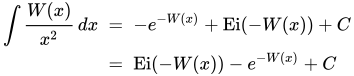
Integrales indefinidas

Introducir variable de sustitución



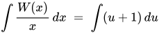
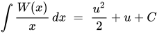


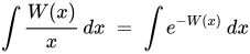
























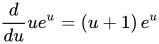
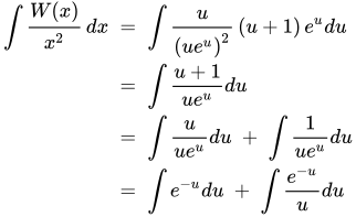
Introduzca la variable de sustitución , que nos da y






Aplicaciones
Resolver ecuaciones
La función W de Lambert se utiliza para resolver ecuaciones en las que la cantidad desconocida se encuentra tanto en la base como en el exponente, o tanto dentro como fuera de un logaritmo. La estrategia consiste en convertir dicha ecuación en una ecuación de la forma ze z = w y luego resolver z utilizando la función W.
Por ejemplo, la ecuación

(donde x es un número real desconocido) se puede resolver reescribiéndolo como
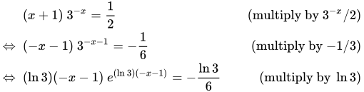
Esta última ecuación tiene la forma deseada y las soluciones para x real son:

y por lo tanto:

Generalmente, la solución a

es:
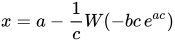
donde a , b y c son constantes complejas, donde b y c no son iguales a cero, y la función W es de cualquier orden entero.
Flujos viscosos
Los frentes y depósitos de flujo granular y de escombros, y los frentes de fluidos viscosos en eventos naturales y en experimentos de laboratorio se pueden describir utilizando la función omega de Lambert-Euler de la siguiente manera:

where H(x) is the debris flow height, x is the channel downstream position, L is the unified model parameter consisting of several physical and geometrical parameters of the flow, flow height and the hydraulic pressure gradient.
In pipe flow, the Lambert W function is part of the explicit formulation of the Colebrook equation for finding the Darcy friction factor. This factor is used to determine the pressure drop through a straight run of pipe when the flow is turbulent.[21]
Time-dependent flow in simple branch hydraulic systems
The principal branch of the Lambert W function is employed in the field of mechanical engineering, in the study of time dependent transfer of Newtonian fluids between two reservoirs with varying free surface levels, using centrifugal pumps.[22] The Lambert W function provided an exact solution to the flow rate of fluid in both the laminar and turbulent regimes: where is the initial flow rate and is time.
![{\displaystyle {\begin{aligned}Q_{\text{turb}}&={\frac {Q_{i}}{\zeta _{i}}}W_{0}\left[\zeta _{i}\,e^{(\zeta _{i}+\beta t/b)}\right]\\Q_{\text{lam}}&={\frac {Q_{i}}{\xi _{i}}}W_{0}\left[\xi _{i}\,e^{\left(\xi _{i}+\beta t/(b-\Gamma _{1})\right)}\right]\end{aligned}}}](https://wikimedia.org/api/rest_v1/media/math/render/svg/43d43eeebc5111975f2588d8a36063fe7a6bfeaa)


Neuroimaging
The Lambert W function is employed in the field of neuroimaging for linking cerebral blood flow and oxygen consumption changes within a brain voxel, to the corresponding blood oxygenation level dependent (BOLD) signal.[23]
Chemical engineering
The Lambert W function is employed in the field of chemical engineering for modeling the porous electrode film thickness in a glassy carbon based supercapacitor for electrochemical energy storage. The Lambert W function provides an exact solution for a gas phase thermal activation process where growth of carbon film and combustion of the same film compete with each other.[24][25]
Crystal growth
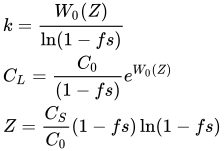
In the crystal growth, the negative principal of the Lambert W-function can be used to calculate the distribution coefficient, , and solute concentration in the melt, ,[26][27] from the Scheil equation:


Materials science
The Lambert W function is employed in the field of epitaxial film growth for the determination of the critical dislocation onset film thickness. This is the calculated thickness of an epitaxial film, where due to thermodynamic principles the film will develop crystallographic dislocations in order to minimise the elastic energy stored in the films. Prior to application of Lambert W for this problem, the critical thickness had to be determined via solving an implicit equation. Lambert W turns it in an explicit equation for analytical handling with ease.[28]
Porous media
The Lambert W function has been employed in the field of fluid flow in porous media to model the tilt of an interface separating two gravitationally segregated fluids in a homogeneous tilted porous bed of constant dip and thickness where the heavier fluid, injected at the bottom end, displaces the lighter fluid that is produced at the same rate from the top end. The principal branch of the solution corresponds to stable displacements while the −1 branch applies if the displacement is unstable with the heavier fluid running underneath the lighter fluid.[29]
Bernoulli numbers and Todd genus
The equation (linked with the generating functions of Bernoulli numbers and Todd genus):

can be solved by means of the two real branches W0 and W−1:

This application shows that the branch difference of the W function can be employed in order to solve other transcendental equations.[30]
Statistics
The centroid of a set of histograms defined with respect to the symmetrized Kullback–Leibler divergence (also called the Jeffreys divergence [31]) has a closed form using the Lambert W function.[32]
Pooling of tests for infectious diseases
Solving for the optimal group size to pool tests so that at least one individual is infected involves the Lambert W function.[33][34][35]
Exact solutions of the Schrödinger equation
The Lambert W function appears in a quantum-mechanical potential, which affords the fifth – next to those of the harmonic oscillator plus centrifugal, the Coulomb plus inverse square, the Morse, and the inverse square root potential – exact solution to the stationary one-dimensional Schrödinger equation in terms of the confluent hypergeometric functions. The potential is given as
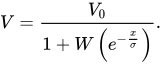
A peculiarity of the solution is that each of the two fundamental solutions that compose the general solution of the Schrödinger equation is given by a combination of two confluent hypergeometric functions of an argument proportional to[36]
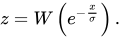
The Lambert W function also appears in the exact solution for the bound state energy of the one dimensional Schrödinger equation with a Double Delta Potential.
Exact solution of QCD coupling constant
In Quantum chromodynamics, the quantum field theory of the Strong interaction, the coupling constant is computed perturbatively, the order n corresponding to Feynman diagrams including n quantum loops.[37] The first order, n=1, solution is exact (at that order) and analytical. At higher orders, n>1, there is no exact and analytical solution and one typically uses an iterative method to furnish an approximate solution. However, for second order, n=2, the Lambert function provides an exact (if non-analytical) solution.[37]

Exact solutions of the Einstein vacuum equations
In the Schwarzschild metric solution of the Einstein vacuum equations, the W function is needed to go from the Eddington–Finkelstein coordinates to the Schwarzschild coordinates. For this reason, it also appears in the construction of the Kruskal–Szekeres coordinates.
Resonances of the delta-shell potential
The s-wave resonances of the delta-shell potential can be written exactly in terms of the Lambert W function.[38]
Thermodynamic equilibrium
If a reaction involves reactants and products having heat capacities that are constant with temperature then the equilibrium constant K obeys
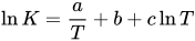
for some constants a, b, and c. When c (equal to ΔCp/R) is not zero the value or values of T can be found where K equals a given value as follows, where L can be used for ln T.
![{\displaystyle {\begin{aligned}-a&=(b-\ln K)T+cT\ln T\\&=(b-\ln K)e^{L}+cLe^{L}\\[5pt]-{\frac {a}{c}}&=\left({\frac {b-\ln K}{c}}+L\right)e^{L}\\[5pt]-{\frac {a}{c}}e^{\frac {b-\ln K}{c}}&=\left(L+{\frac {b-\ln K}{c}}\right)e^{L+{\frac {b-\ln K}{c}}}\\[5pt]L&=W\left(-{\frac {a}{c}}e^{\frac {b-\ln K}{c}}\right)+{\frac {\ln K-b}{c}}\\[5pt]T&=\exp \left(W\left(-{\frac {a}{c}}e^{\frac {b-\ln K}{c}}\right)+{\frac {\ln K-b}{c}}\right).\end{aligned}}}](https://wikimedia.org/api/rest_v1/media/math/render/svg/3eb5cee9fdd7908a30ded5a772ec49f985ebaa1a)
If a and c have the same sign there will be either two solutions or none (or one if the argument of W is exactly −1/e). (The upper solution may not be relevant.) If they have opposite signs, there will be one solution.
Phase separation of polymer mixtures
In the calculation of the phase diagram of thermodynamically incompatible polymer mixtures according to the Edmond-Ogston model, the solutions for binodal and tie-lines are formulated in terms of Lambert W functions.[39]
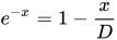
Wien's displacement law in a D-dimensional universe
Wien's displacement law is expressed as . With and , where is the spectral energy energy density, one finds , where is the number of degrees of freedom for spatial translation. The solution shows that the spectral energy density is dependent on the dimensionality of the universe.[40]






AdS/CFT correspondence
The classical finite-size corrections to the dispersion relations of giant magnons, single spikes and GKP strings can be expressed in terms of the Lambert W function.[41][42]
Epidemiology
In the t → ∞ limit of the SIR model, the proportion of susceptible and recovered individuals has a solution in terms of the Lambert W function.[43]
Determination of the time of flight of a projectile
The total time of the journey of a projectile which experiences air resistance proportional to its velocity can be determined in exact form by using the Lambert W function.
Electromagnetic surface wave propagation
The transcendental equation that appears in the determination of the propagation wave number of an electromagnetic axially symmetric surface wave (a low-attenuation single TM01 mode) propagating in a cylindrical metallic wire gives rise to an equation like u ln u = v (where u and v clump together the geometrical and physical factors of the problem), which is solved by the Lambert W function. The first solution to this problem, due to Sommerfeld circa 1898, already contained an iterative method to determine the value of the Lambert W function.[44]
Orthogonal trajectories of real ellipses
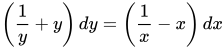
The family of ellipses centered at is parameterized by eccentricity . The orthogonal trajectories of this family are given by the differential equation whose general solution is the family .





Generalizations
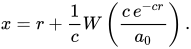
The standard Lambert W function expresses exact solutions to transcendental algebraic equations (in x) of the form:
where a0, c and r are real constants. The solution is Generalizations of the Lambert W function[45][46][47] include:
- An application to general relativity and quantum mechanics (quantum gravity) in lower dimensions, in fact a link (unknown prior to 2007[48]) between these two areas, where the right-hand side of (1) is replaced by a quadratic polynomial in x:
where r1 and r2 are real distinct constants, the roots of the quadratic polynomial. Here, the solution is a function which has a single argument x but the terms like ri and a0 are parameters of that function. In this respect, the generalization resembles the hypergeometric function and the Meijer G function but it belongs to a different class of functions. When r1 = r2, both sides of (2) can be factored and reduced to (1) and thus the solution reduces to that of the standard W function. Equation (2) expresses the equation governing the dilaton field, from which is derived the metric of the R = T or lineal two-body gravity problem in 1 + 1 dimensions (one spatial dimension and one time dimension) for the case of unequal rest masses, as well as the eigenenergies of the quantum-mechanical double-well Dirac delta function model for unequal charges in one dimension.
- Analytical solutions of the eigenenergies of a special case of the quantum mechanical three-body problem, namely the (three-dimensional) hydrogen molecule-ion.[49] Here the right-hand side of (1) is replaced by a ratio of infinite order polynomials in x:
where ri and si are distinct real constants and x is a function of the eigenenergy and the internuclear distance R. Equation (3) with its specialized cases expressed in (1) and (2) is related to a large class of delay differential equations. G. H. Hardy's notion of a "false derivative" provides exact multiple roots to special cases of (3).[50]
Applications of the Lambert W function in fundamental physical problems are not exhausted even for the standard case expressed in (1) as seen recently in the area of atomic, molecular, and optical physics.[51]
Plots
- Plots of the Lambert W function on the complex plane
-
 z = Re(W0(x + iy))
 -
 z = Im(W0(x + iy))
 -
 z = |W0(x + iy)|
 -
 Superimposition of the previous three plots


Numerical evaluation
The W function may be approximated using Newton's method, with successive approximations to w = W(z) (so z = wew) being

The W function may also be approximated using Halley's method,

given in Corless et al.[3] to compute W.
For real , it may be approximated by the quadratic-rate recursive formula of R. Iacono and J.P. Boyd:[12]

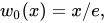
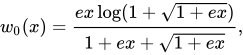
Lajos Lóczi proves[52] that by using this iteration with an appropriate starting value ,

- For the principal branch
- if :
- if
- if
- For the branch
- if
- if








![{\displaystyle x\in (-1/e,-1/4]:}](https://wikimedia.org/api/rest_v1/media/math/render/svg/24b94a22ce7703c01fad21e3dc02064c914fb7aa)

one can determine the maximum number of iteration steps in advance for any precision:
- if (Theorem 2.4):
- if (Theorem 2.9):
- if
- for the principal branch (Theorem 2.17):
- for the branch (Theorem 2.23):







Toshio Fukushima has presented a fast method for approximating the real valued parts of the principal and secondary branches of the W function without using any iteration.[53] In this method the W function is evaluated as a conditional switch of rational functions on transformed varibles:
where x, u, y and v are transformations of z:


.

Here , , , and are rational functions whose coefficients for different k-values are listed in the referenced paper together with the values that determine the subdomains. With higher degree polynomials in these rational functions the method can approximate the W function more accurately.


For example, when , can be approximated to 24 bits of accuracy on 64-bit floating point values as where x is defined with the transformation above and the coefficients and are given in the table below.


Fukushima also offers an approximation with 50 bits of accuracy on 64-bit floats that uses 8th and 7th degree polynomials.
Software
The Lambert W function is implemented in many programming languages. Some of them are listed below:
C++ code for all the branches of the complex Lambert W function is also available on the homepage of István Mező.[65]
See also
- Wright omega function
- Lambert's trinomial equation
- Lagrange inversion theorem
- Experimental mathematics
- Holstein–Herring method
- R = T model
- Ross' π lemma
Notes
- ^ Lehtonen, Jussi (April 2016), Rees, Mark (ed.), "The Lambert W function in ecological and evolutionary models", Methods in Ecology and Evolution, 7 (9): 1110–1118, Bibcode:2016MEcEv...7.1110L, doi:10.1111/2041-210x.12568, S2CID 124111881
- ^ Chow, Timothy Y. (1999), "What is a closed-form number?", American Mathematical Monthly, 106 (5): 440–448, arXiv:math/9805045, doi:10.2307/2589148, JSTOR 2589148, MR 1699262.
- ^ a b c d e Corless, R. M.; Gonnet, G. H.; Hare, D. E. G.; Jeffrey, D. J.; Knuth, D. E. (1996). "On the LambertW function" (PDF). Advances in Computational Mathematics. 5: 329–359. doi:10.1007/BF02124750. S2CID 29028411.
- ^ Lambert J. H., "Observationes variae in mathesin puram", Acta Helveticae physico-mathematico-anatomico-botanico-medica, Band III, 128–168, 1758.
- ^ Euler, L. "De serie Lambertina Plurimisque eius insignibus proprietatibus". Acta Acad. Scient. Petropol. 2, 29–51, 1783. Reprinted in Euler, L. Opera Omnia, Series Prima, Vol. 6: Commentationes Algebraicae. Leipzig, Germany: Teubner, pp. 350–369, 1921.
- ^ Scott, TC; Babb, JF; Dalgarno, A; Morgan, John D (Aug 15, 1993). "The calculation of exchange forces: General results and specific models". J. Chem. Phys. 99 (4). American Institute of Physics: 2841–2854. Bibcode:1993JChPh..99.2841S. doi:10.1063/1.465193. ISSN 0021-9606.
- ^ Corless, R. M.; Gonnet, G. H.; Hare, D. E. G.; Jeffrey, D. J. (1993). "Lambert's function in Maple". The Maple Technical Newsletter. 9: 12–22. CiteSeerX 10.1.1.33.2556.
- ^ Mező, István (2022). The Lambert W Function: Its Generalizations and Applications. doi:10.1201/9781003168102. ISBN 9781003168102. S2CID 247491347.
- ^ Bronstein, Manuel; Corless, Robert M.; Davenport, James H.; Jeffrey, D. J. (2008). "Algebraic properties of the Lambert W {\displaystyle W} function from a result of Rosenlicht and of Liouville" (PDF). Integral Transforms and Special Functions. 19 (10): 709–712. doi:10.1080/10652460802332342. S2CID 120069437. Archived (PDF) from the original on 2015-12-11.
- ^ A. Hoorfar, M. Hassani, Inequalities on the Lambert W Function and Hyperpower Function, JIPAM, Theorem 2.7, page 7, volume 9, issue 2, article 51. 2008.
- ^ Chatzigeorgiou, I. (2013). "Bounds on the Lambert function and their Application to the Outage Analysis of User Cooperation". IEEE Communications Letters. 17 (8): 1505–1508. arXiv:1601.04895. doi:10.1109/LCOMM.2013.070113.130972. S2CID 10062685.
- ^ a b Iacono, Roberto; Boyd, John P. (2017-12-01). "New approximations to the principal real-valued branch of the Lambert W-function". Advances in Computational Mathematics. 43 (6): 1403–1436. doi:10.1007/s10444-017-9530-3. ISSN 1572-9044. S2CID 254184098.
- ^ "Lambert function: Identities (formula 01.31.17.0001)".
- ^ "Lambert W-Function".
- ^ https://isa-afp.org/entries/Lambert_W.html Note: although one of the assumptions of the relevant lemma states that x must be > 1/e, inspection of said lemma reveals that this assumption is unused. The lower bound is in fact x > 0. The reason for the branch switch at e is simple: for x > 1 there are always two solutions, −ln x and another one that you'd get from the x on the other side of e that would feed the same value to W; these must crossover at x = e: [1] Wn cannot distinguish a value of ln x/x from an x < e from the same value from the other x > e, so it cannot flip the order of its return values.
- ^ Finch, S. R. (2003). Mathematical constants. Cambridge University Press. p. 450.
- ^ Kalugin, German A.; Jeffrey, David J.; Corless, Robert M. (2012). "Bernstein, Pick, Poisson and related integral expressions for Lambert W" (PDF). Integral Transforms and Special Functions. 23 (11): 817–829. doi:10.1080/10652469.2011.640327. MR 2989751. See Theorem 3.4, p. 821 of published version (p. 5 of preprint).
- ^ Dubinov, A. E.; Dubinova, I. D.; Saǐkov, S. K. (2006). The Lambert W Function and Its Applications to Mathematical Problems of Physics (in Russian). RFNC-VNIIEF. p. 53.
- ^ Robert M., Corless; David J., Jeffrey; Donald E., Knuth (1997). "A sequence of series for the Lambert W function". Proceedings of the 1997 international symposium on Symbolic and algebraic computation - ISSAC '97. pp. 197–204. doi:10.1145/258726.258783. ISBN 978-0897918756. S2CID 6274712.
- ^ "The Lambert W Function". Ontario Research Centre for Computer Algebra.
- ^ More, A. A. (2006). "Analytical solutions for the Colebrook and White equation and for pressure drop in ideal gas flow in pipes". Chemical Engineering Science. 61 (16): 5515–5519. Bibcode:2006ChEnS..61.5515M. doi:10.1016/j.ces.2006.04.003.
- ^ Pellegrini, C. C.; Zappi, G. A.; Vilalta-Alonso, G. (2022-05-12). "An Analytical Solution for the Time-Dependent Flow in Simple Branch Hydraulic Systems with Centrifugal Pumps". Arabian Journal for Science and Engineering. 47 (12): 16273–16287. doi:10.1007/s13369-022-06864-9. ISSN 2193-567X. S2CID 248762601.
- ^ Sotero, Roberto C.; Iturria-Medina, Yasser (2011). "From Blood oxygenation level dependent (BOLD) signals to brain temperature maps". Bull Math Biol (Submitted manuscript). 73 (11): 2731–47. doi:10.1007/s11538-011-9645-5. PMID 21409512. S2CID 12080132.
- ^ Braun, Artur; Wokaun, Alexander; Hermanns, Heinz-Guenter (2003). "Analytical Solution to a Growth Problem with Two Moving Boundaries". Appl Math Model. 27 (1): 47–52. doi:10.1016/S0307-904X(02)00085-9.
- ^ Braun, Artur; Baertsch, Martin; Schnyder, Bernhard; Koetz, Ruediger (2000). "A Model for the film growth in samples with two moving boundaries – An Application and Extension of the Unreacted-Core Model". Chem Eng Sci. 55 (22): 5273–5282. doi:10.1016/S0009-2509(00)00143-3.
- ^ Asadian, M; Saeedi, H; Yadegari, M; Shojaee, M (June 2014). "Determinations of equilibrium segregation, effective segregation and diffusion coefficients for Nd+3 doped in molten YAG". Journal of Crystal Growth. 396 (15): 61–65. Bibcode:2014JCrGr.396...61A. doi:10.1016/j.jcrysgro.2014.03.028. https://doi.org/10.1016/j.jcrysgro.2014.03.028
- ^ Asadian, M; Zabihi, F; Saeedi, H (March 2024). "Segregation and constitutional supercooling in Nd:YAG Czochralski crystal growth". Journal of Crystal Growth. 630: 127605. Bibcode:2024JCrGr.63027605A. doi:10.1016/j.jcrysgro.2024.127605. S2CID 267414096. https://doi.org/10.1016/j.jcrysgro.2024.127605
- ^ Braun, Artur; Briggs, Keith M.; Boeni, Peter (2003). "Analytical solution to Matthews' and Blakeslee's critical dislocation formation thickness of epitaxially grown thin films". J Cryst Growth. 241 (1–2): 231–234. Bibcode:2002JCrGr.241..231B. doi:10.1016/S0022-0248(02)00941-7.
- ^ Colla, Pietro (2014). "A New Analytical Method for the Motion of a Two-Phase Interface in a Tilted Porous Medium". PROCEEDINGS, Thirty-Eighth Workshop on Geothermal Reservoir Engineering, Stanford University. SGP-TR-202.([2])
- ^ D. J. Jeffrey and J. E. Jankowski, "Branch differences and Lambert W"
- ^ Flavia-Corina Mitroi-Symeonidis; Ion Anghel; Shigeru Furuichi (2019). "Encodings for the calculation of the permutation hypoentropy and their applications on full-scale compartment fire data". Acta Technica Napocensis. 62, IV: 607–616.
- ^ F. Nielsen, "Jeffreys Centroids: A Closed-Form Expression for Positive Histograms and a Guaranteed Tight Approximation for Frequency Histograms"
- ^ https://arxiv.org/abs/2005.03051 J. Batson et al., "A COMPARISON OF GROUP TESTING ARCHITECTURES FOR COVID-19 TESTING".
- ^ A.Z. Broder, "A Note on Double Pooling Tests".
- ^ Rudolf Hanel, Stefan Thurner (2020). "Boosting test-efficiency by pooled testing for SARS-CoV-2—Formula for optimal pool size". PLOS ONE. 15, 11 (11): e0240652. Bibcode:2020PLoSO..1540652H. doi:10.1371/journal.pone.0240652. PMC 7641378. PMID 33147228.
- ^ A.M. Ishkhanyan, "The Lambert W barrier – an exactly solvable confluent hypergeometric potential".
- ^ a b Deur, Alexandre; Brodsky, Stanley J.; De Téramond, Guy F. (2016). "The QCD running coupling". Progress in Particle and Nuclear Physics. 90: 1–74. arXiv:1604.08082. Bibcode:2016PrPNP..90....1D. doi:10.1016/j.ppnp.2016.04.003. S2CID 118854278.
- ^ de la Madrid, R. (2017). "Numerical calculation of the decay widths, the decay constants, and the decay energy spectra of the resonances of the delta-shell potential". Nucl. Phys. A. 962: 24–45. arXiv:1704.00047. Bibcode:2017NuPhA.962...24D. doi:10.1016/j.nuclphysa.2017.03.006. S2CID 119218907.
- ^ Bot, A.; Dewi, B.P.C.; Venema, P. (2021). "Phase-separating binary polymer mixtures: the degeneracy of the virial coefficients and their extraction from phase diagrams". ACS Omega. 6 (11): 7862–7878. doi:10.1021/acsomega.1c00450. PMC 7992149. PMID 33778298.
- ^ Cardoso, T. R.; de Castro, A. S. (2005). "The blackbody radiation in a D-dimensional universe". Rev. Bras. Ens. Fis. 27 (4): 559–563. doi:10.1590/S1806-11172005000400007. hdl:11449/211894.
- ^ Floratos, Emmanuel; Georgiou, George; Linardopoulos, Georgios (2014). "Large-Spin Expansions of GKP Strings". JHEP. 2014 (3): 0180. arXiv:1311.5800. Bibcode:2014JHEP...03..018F. doi:10.1007/JHEP03(2014)018. S2CID 53355961.
- ^ Floratos, Emmanuel; Linardopoulos, Georgios (2015). "Large-Spin and Large-Winding Expansions of Giant Magnons and Single Spikes". Nucl. Phys. B. 897: 229–275. arXiv:1406.0796. Bibcode:2015NuPhB.897..229F. doi:10.1016/j.nuclphysb.2015.05.021. S2CID 118526569.
- ^ Wolfram Research, Inc. "Mathematica, Version 12.1". Champaign IL, 2020.
- ^ Mendonça, J. R. G. (2019). "Electromagnetic surface wave propagation in a metallic wire and the Lambert W function". American Journal of Physics. 87 (6): 476–484. arXiv:1812.07456. Bibcode:2019AmJPh..87..476M. doi:10.1119/1.5100943. S2CID 119661071.
- ^ Scott, T. C.; Mann, R. B.; Martinez Ii, Roberto E. (2006). "General Relativity and Quantum Mechanics: Towards a Generalization of the Lambert W Function". AAECC (Applicable Algebra in Engineering, Communication and Computing). 17 (1): 41–47. arXiv:math-ph/0607011. Bibcode:2006math.ph...7011S. doi:10.1007/s00200-006-0196-1. S2CID 14664985.
- ^ Scott, T. C.; Fee, G.; Grotendorst, J. (2013). "Asymptotic series of Generalized Lambert W Function". SIGSAM (ACM Special Interest Group in Symbolic and Algebraic Manipulation). 47 (185): 75–83. doi:10.1145/2576802.2576804. S2CID 15370297.
- ^ Scott, T. C.; Fee, G.; Grotendorst, J.; Zhang, W.Z. (2014). "Numerics of the Generalized Lambert W Function". SIGSAM. 48 (1/2): 42–56. doi:10.1145/2644288.2644298. S2CID 15776321.
- ^ Farrugia, P. S.; Mann, R. B.; Scott, T. C. (2007). "N-body Gravity and the Schrödinger Equation". Class. Quantum Grav. 24 (18): 4647–4659. arXiv:gr-qc/0611144. Bibcode:2007CQGra..24.4647F. doi:10.1088/0264-9381/24/18/006. S2CID 119365501.
- ^ Scott, T. C.; Aubert-Frécon, M.; Grotendorst, J. (2006). "New Approach for the Electronic Energies of the Hydrogen Molecular Ion". Chem. Phys. 324 (2–3): 323–338. arXiv:physics/0607081. Bibcode:2006CP....324..323S. CiteSeerX 10.1.1.261.9067. doi:10.1016/j.chemphys.2005.10.031. S2CID 623114.
- ^ Maignan, Aude; Scott, T. C. (2016). "Fleshing out the Generalized Lambert W Function". SIGSAM. 50 (2): 45–60. doi:10.1145/2992274.2992275. S2CID 53222884.
- ^ Scott, T. C.; Lüchow, A.; Bressanini, D.; Morgan, J. D. III (2007). "The Nodal Surfaces of Helium Atom Eigenfunctions" (PDF). Phys. Rev. A. 75 (6): 060101. Bibcode:2007PhRvA..75f0101S. doi:10.1103/PhysRevA.75.060101. hdl:11383/1679348. Archived (PDF) from the original on 2017-09-22.
- ^ Lóczi, Lajos (2022-11-15). "Guaranteed- and high-precision evaluation of the Lambert W function". Applied Mathematics and Computation. 433: 127406. doi:10.1016/j.amc.2022.127406. hdl:10831/89771. ISSN 0096-3003.
- ^ Fukushima, Toshio (2020-11-25). "Precise and fast computation of Lambert W function by piecewise minimax rational function approximation with variable transformation". doi:10.13140/RG.2.2.30264.37128.
- ^ "LambertW - Maple Help".
- ^ lambertw – MATLAB
- ^ "lambertw - specfun on Octave-Forge". Retrieved 2024-09-12.
- ^ Maxima, a Computer Algebra System
- ^ ProductLog - Wolfram Language Reference
- ^ "Scipy.special.lambertw — SciPy v0.16.1 Reference Guide".
- ^ ntheory - MetaCPAN
- ^ "Lambert W Functions - GNU Scientific Library (GSL)".
- ^ "Lambert W function - Boost libraries".
- ^ Adler, Avraham (2017-04-24), lamW: Lambert W Function, retrieved 2017-12-19
- ^ Sörngård, Johanna (2024-07-28), lambert_w, retrieved 2024-09-11
- ^ István Mező - Personal webpage
References
- Corless, R.; Gonnet, G.; Hare, D.; Jeffrey, D.; Knuth, Donald (1996). "On the Lambert W function" (PDF). Advances in Computational Mathematics. 5: 329–359. doi:10.1007/BF02124750. ISSN 1019-7168. S2CID 29028411. Archived from the original (PDF) on 2010-12-14. Retrieved 2007-03-10.
- Chapeau-Blondeau, F.; Monir, A. (2002). "Evaluation of the Lambert W Function and Application to Generation of Generalized Gaussian Noise With Exponent 1/2" (PDF). IEEE Trans. Signal Process. 50 (9). doi:10.1109/TSP.2002.801912. Archived from the original (PDF) on 2012-03-28. Retrieved 2004-03-10.
- Francis; et al. (2000). "Quantitative General Theory for Periodic Breathing". Circulation. 102 (18): 2214–21. CiteSeerX 10.1.1.505.7194. doi:10.1161/01.cir.102.18.2214. PMID 11056095. S2CID 14410926.(La función de Lambert se utiliza para resolver la dinámica diferencial de retardo en enfermedades humanas).
- Hayes, B. (2005). "¿Por qué W?" (PDF) . American Scientist . 93 (2): 104–108. doi :10.1511/2005.2.104. Archivado (PDF) desde el original el 10 de octubre de 2022.
- Roy, R.; Olver, FWJ (2010), "Función W de Lambert", en Olver, Frank WJ ; Lozier, Daniel M.; Boisvert, Ronald F.; Clark, Charles W. (eds.), Manual del NIST de funciones matemáticas , Cambridge University Press, ISBN 978-0-521-19225-5, Sr. 2723248.
- Stewart, Seán M. (2005). "¿Una nueva función elemental para nuestros currículos?" (PDF) . Revista australiana de matemáticas para estudiantes de último año . 19 (2): 8–26. ISSN 0819-4564. Archivado (PDF) desde el original el 10 de octubre de 2022.
- Veberic, D., "Divirtiéndose con la función W(x) de Lambert" arXiv:1003.1628 (2010); Veberic, D. (2012). " Función W de Lambert para aplicaciones en física". Computer Physics Communications . 183 (12): 2622–2628. arXiv : 1209.0735 . Bibcode :2012CoPhC.183.2622V. doi :10.1016/j.cpc.2012.07.008. S2CID 315088.
- Chatzigeorgiou, I. (2013). "Límites de la función Lambert y su aplicación al análisis de interrupciones de la cooperación del usuario". IEEE Communications Letters . 17 (8): 1505–1508. arXiv : 1601.04895 . doi :10.1109/LCOMM.2013.070113.130972. S2CID 10062685.
Enlaces externos

- Biblioteca digital del Instituto Nacional de Ciencia y Tecnología – Lambert W
- MathWorld – Función W de Lambert
- Cálculo de la función W de Lambert
- Corless et al. Notas sobre la investigación de Lambert W.
- Implementación de C++ GPL con iteración de Halley y Fritsch.
- Funciones especiales de la biblioteca científica GNU – GSL
- [3]