 Hispanopedia Wiki
In mathematics and computational science, the Euler method (also called the forward Euler method) is a first-order numerical procedure for solving ordinary differential equations (ODEs) with a given initial value. It is the most basic explicit method for numerical integration of ordinary differential equations and is the simplest Runge–Kutta method. The Euler method is named after Leonhard Euler, who first proposed it in his book Institutionum calculi integralis (published 1768–1770).[1]
The Euler method is a first-order method, which means that the local error (error per step) is proportional to the square of the step size, and the global error (error at a given time) is proportional to the step size. The Euler method often serves as the basis to construct more complex methods, e.g., predictor–corrector method.
Geometrical description
Purpose and why it works
Consider the problem of calculating the shape of an unknown curve which starts at a given point and satisfies a given differential equation. Here, a differential equation can be thought of as a formula by which the slope of the tangent line to the curve can be computed at any point on the curve, once the position of that point has been calculated.
The idea is that while the curve is initially unknown, its starting point, which we denote by is known (see Figure 1). Then, from the differential equation, the slope to the curve at can be computed, and so, the tangent line.


Take a small step along that tangent line up to a point Along this small step, the slope does not change too much, so will be close to the curve. If we pretend that is still on the curve, the same reasoning as for the point above can be used. After several steps, a polygonal curve () is computed. In general, this curve does not diverge too far from the original unknown curve, and the error between the two curves can be made small if the step size is small enough and the interval of computation is finite.[2]


First-order process
When given the values for and , and the derivative of is a given function of and denoted as . Begin the process by setting . Next, choose a value for the size of every step along t-axis, and set (or equivalently ). Now, the Euler method is used to find from and :[3]







The value of is an approximation of the solution at time , i.e., . The Euler method is explicit, i.e. the solution is an explicit function of for .


Higher-order process
While the Euler method integrates a first-order ODE, any ODE of order can be represented as a system of first-order ODEs. When given the ODE of order defined as


as well as , , and , we implement the following formula until we reach the approximation of the solution to the ODE at the desired time:
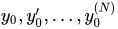

These first-order systems can be handled by Euler's method or, in fact, by any other scheme for first-order systems.[4]
First-order example
Given the initial value problem

we would like to use the Euler method to approximate .[5]

Using step size equal to 1 (h = 1)




The Euler method is
so first we must compute . In this simple differential equation, the function is defined by . We have



By doing the above step, we have found the slope of the line that is tangent to the solution curve at the point . Recall that the slope is defined as the change in divided by the change in , or .


The next step is to multiply the above value by the step size , which we take equal to one here:

Since the step size is the change in , when we multiply the step size and the slope of the tangent, we get a change in value. This value is then added to the initial value to obtain the next value to be used for computations.

The above steps should be repeated to find , and .


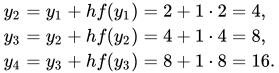
Due to the repetitive nature of this algorithm, it can be helpful to organize computations in a chart form, as seen below, to avoid making errors.
The conclusion of this computation is that . The exact solution of the differential equation is , so . Although the approximation of the Euler method was not very precise in this specific case, particularly due to a large value step size , its behaviour is qualitatively correct as the figure shows.



Using other step sizes


As suggested in the introduction, the Euler method is more accurate if the step size is smaller. The table below shows the result with different step sizes. The top row corresponds to the example in the previous section, and the second row is illustrated in the figure.
The error recorded in the last column of the table is the difference between the exact solution at and the Euler approximation. In the bottom of the table, the step size is half the step size in the previous row, and the error is also approximately half the error in the previous row. This suggests that the error is roughly proportional to the step size, at least for fairly small values of the step size. This is true in general, also for other equations; see the section Global truncation error for more details.

Other methods, such as the midpoint method also illustrated in the figures, behave more favourably: the global error of the midpoint method is roughly proportional to the square of the step size. For this reason, the Euler method is said to be a first-order method, while the midpoint method is second order.
We can extrapolate from the above table that the step size needed to get an answer that is correct to three decimal places is approximately 0.00001, meaning that we need 400,000 steps. This large number of steps entails a high computational cost. For this reason, higher-order methods are employed such as Runge–Kutta methods or linear multistep methods, especially if a high accuracy is desired.[6]
Higher-order example
For this third-order example, assume that the following information is given:
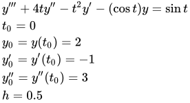
A partir de esto podemos aislar y ''' para obtener la ecuación:

Usando eso podemos obtener la solución para: Y utilizando la solución para, podemos obtener la solución para:Podemos continuar este proceso utilizando la misma fórmula durante el tiempo que sea necesario para encontrar cualquiera.deseado.

![{\displaystyle {\begin{aligned}{\vec {y}}_{1}&={\begin{pmatrix}y_{1}\\y_{1}'\\y_{1}''\end{pmatrix}}={\begin{pmatrix}y_{0}\\y'_{0}\\y''_{0}\end{pmatrix}}+h{\begin{pmatrix}y'_{0}\\y''_{0}\\f{\left(t_{0},y_{0},y'_{0},y''_{0}\right)}\end{pmatrix}}\\[1ex]&={\begin{pmatrix}2\\-1\\3\end{pmatrix}}+0.5\cdot {\begin{pmatrix}-1\\3\\\sin {0}+(\cos {0})\cdot 2+0^{2}\cdot (-1)-4\cdot 0\cdot 3\end{pmatrix}}\\[1ex]&={\begin{pmatrix}1.5\\0.5\\4\end{pmatrix}}\end{aligned}}}](https://wikimedia.org/api/rest_v1/media/math/render/svg/12d39d9f7b06f2891cd612caf12d43f1895a4c97)

![{\displaystyle {\begin{aligned}{\vec {y}}_{2}&={\begin{pmatrix}y_{2}\\y_{2}'\\y_{2}''\end{pmatrix}}={\begin{pmatrix}y_{1}\\y'_{1}\\y''_{1}\end{pmatrix}}+h{\begin{pmatrix}y'_{1}\\y''_{1}\\f{\left(t_{1},y_{1},y'_{1},y''_{1}\right)}\end{pmatrix}}\\[1ex]&={\begin{pmatrix}1.5\\0.5\\4\end{pmatrix}}+0.5\cdot {\begin{pmatrix}0.5\\4\\\sin {0.5}+(\cos {0.5})\cdot 1.5+0.5^{2}\cdot 0.5-4\cdot 0.5\cdot 4\end{pmatrix}}\\[1ex]&={\begin{pmatrix}1.75\\2.5\\0.9604...\end{pmatrix}}\end{aligned}}}](https://wikimedia.org/api/rest_v1/media/math/render/svg/b2977cf7737e8f5d2bf33689bc668c308ce85f14)

Derivación
El método de Euler se puede derivar de varias maneras.
- En primer lugar, está la descripción geométrica anterior.
- Otra posibilidad es considerar el desarrollo de Taylor de la funciónalrededor: La ecuación diferencial establece queSi esto se sustituye en el desarrollo de Taylor y se ignoran los términos cuadráticos y de orden superior, surge el método de Euler. [ 7 ] El desarrollo de Taylor se utiliza a continuación para analizar el error cometido por el método de Euler, y puede extenderse para producir métodos de Runge-Kutta .
- Una derivación estrechamente relacionada consiste en sustituir la fórmula de diferencias finitas hacia adelante por la derivada, en la ecuación diferencial. Nuevamente, esto produce el método de Euler. [ 8 ] Un cálculo similar conduce al método del punto medio y al método de Euler hacia atrás .
- Finalmente, se puede integrar la ecuación diferencial desdeay aplicamos el teorema fundamental del cálculo para obtener: Ahora aproximemos la integral mediante el método del rectángulo de la izquierda (con un solo rectángulo): Combinando ambas ecuaciones, se obtiene nuevamente el método de Euler. [ 9 ]


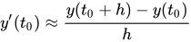


Esta línea de pensamiento puede continuarse para llegar a varios métodos lineales de múltiples pasos .
Error de truncamiento local
El error de truncamiento local del método de Euler es el error cometido en un solo paso. Es la diferencia entre la solución numérica después de un paso,y la solución exacta en ese momentoLa solución numérica viene dada por



Para obtener la solución exacta, utilizamos el desarrollo de Taylor mencionado en la sección Derivación anterior:

El error de truncamiento local (LTE) introducido por el método de Euler viene dado por la diferencia entre estas ecuaciones:

Este resultado es válido sitiene una tercera derivada acotada. [ 10 ]
Esto demuestra que para pequeños, el error de truncamiento local es aproximadamente proporcional aEsto hace que el método de Euler sea menos preciso que las técnicas de orden superior, como los métodos de Runge-Kutta y los métodos lineales de pasos múltiples , para los cuales el error de truncamiento local es proporcional a una potencia mayor del tamaño del paso.

Se puede obtener una formulación ligeramente diferente para el error de truncamiento local utilizando la forma de Lagrange para el término restante en el teorema de Taylor . Sitiene una segunda derivada continua, entonces existe unade tal manera que [ 11 ]
![{\displaystyle \xi \in [t_{0},t_{0}+h]}](https://wikimedia.org/api/rest_v1/media/math/render/svg/21216efa1ba4d1d6558385ff51b38a37f3ffc42f)

En las expresiones anteriores para el error, la segunda derivada de la solución exacta desconocidapuede ser reemplazado por una expresión que involucre el lado derecho de la ecuación diferencial. De hecho, se deduce de la ecuaciónque [ 12 ]

Error de truncamiento global
El error de truncamiento global es el error en un tiempo fijo., después de la cantidad de pasos que el método necesite tomar para llegar a ese tiempo desde el tiempo inicial. El error de truncamiento global es el efecto acumulativo de los errores de truncamiento locales cometidos en cada paso. [ 13 ] El número de pasos se determina fácilmente como, que es proporcional ay el error cometido en cada paso es proporcional a(véase la sección anterior). Por lo tanto, cabe esperar que el error de truncamiento global sea proporcional a. [ 14 ]


Este razonamiento intuitivo se puede precisar. Si la solucióntiene una segunda derivada acotada yes Lipschitz continua en su segundo argumento, entonces el error de truncamiento global (denotado como) está delimitado por


dóndees una cota superior para la segunda derivada deen el intervalo dado yes la constante de Lipschitz de. [ 15 ] O más simplemente, cuando, el valor(de tal manera quese trata como una constante). En cambio,donde funciónes la solución exacta que solo contiene lavariable.


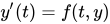
![{\textstyle L={\text{max}}\left(|{\frac {d}{dy}}\left[f(t,y)\right]|\right)}](https://wikimedia.org/api/rest_v1/media/math/render/svg/918c33596aaf1730984ce5857ee16c113dbd1bb4)
![{\textstyle M=\max \left(\left|{\frac {d^{2}}{dt^{2}}}\left[y(t)\right]\right|\right)}](https://wikimedia.org/api/rest_v1/media/math/render/svg/0d7390889a132e632a6f49b7a3e07a4638d63817)

La forma precisa de esta cota tiene poca importancia práctica, ya que en la mayoría de los casos la cota sobreestima enormemente el error real cometido por el método de Euler. [ 16 ] Lo importante es que muestra que el error de truncamiento global es (aproximadamente) proporcional aPor esta razón, se dice que el método de Euler es de primer orden. [ 17 ]
Ejemplo
Si tenemos la ecuación diferencialy la solución exactay queremos encontrarypara cuando. De esta forma podemos hallar el límite de error en t = 2,5 y h = 0,5:

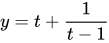

![{\displaystyle {\begin{aligned}L&=\max \left|{\frac {d}{dy}}f(t,y)\right|=\max _{2\leq t\leq 3}\left|{\frac {d}{dy}}\left[1+\left(ty\right)^{2}\right]\right|\\[1ex]&=\max _{2\leq t\leq 3}\left|2\left(ty\right)\right|=\max _{2\leq t\leq 3}\left|2\left(t-\left[t+{\frac {1}{t-1}}\right]\right)\right|\\[1ex]&=\max _{2\leq t\leq 3}\left|-{\frac {2}{t-1}}\right|=2\end{aligned}}}](https://wikimedia.org/api/rest_v1/media/math/render/svg/06b0eee0130d84eded626517c689bb00244b5b06)
![{\displaystyle {\begin{aligned}M&=\max \left|{\frac {d^{2}}{dt^{2}}}\left[y(t)\right]\right|\\&=\max _{2\leq t\leq 3}\left|{\frac {d^{2}}{dt^{2}}}\left(t+{\frac {1}{1-t}}\right)\right|\\&=\max _{2\leq t\leq 3}\left|{\frac {2}{\left(-t+1\right)^{3}}}\right|=2\end{aligned}}}](https://wikimedia.org/api/rest_v1/media/math/render/svg/7f40aadeb1ff24778f87c6b1b8bf32cbf55f8bf9)
Nótese que t 0 es igual a 2 porque es el límite inferior para t en.
![{\displaystyle {\begin{aligned}{\text{límite de error}}&={\frac {hM}{2L}}\left(e^{L(t_{i}-t_{0})}-1\right)\\[1ex]&={\frac {0.5\cdot 2}{2\cdot 2}}\left(e^{2(2.5-2)}-1\right)=0.42957\end{aligned}}}](https://wikimedia.org/api/rest_v1/media/math/render/svg/65ddc6a993d9eee4e821c97a268269ca8890e1b4)
Estabilidad numérica


The Euler method can also be numerically unstable, especially for stiff equations, meaning that the numerical solution grows very large for equations where the exact solution does not. This can be illustrated using the linear equation The exact solution is , which decays to zero as . However, if the Euler method is applied to this equation with step size , then the numerical solution is qualitatively wrong: It oscillates and grows (see the figure). This is what it means to be unstable. If a smaller step size is used, for instance , then the numerical solution does decay to zero.



If the Euler method is applied to the linear equation , then the numerical solution is unstable if the product is outside the region illustrated on the right. This region is called the (linear) stability region.[18] In the example, , so if then which is outside the stability region, and thus the numerical solution is unstable.


This limitation — along with its slow convergence of error with — means that the Euler method is not often used, except as a simple example of numerical integration. Frequently models of physical systems contain terms representing fast-decaying elements (i.e. with large negative exponential arguments). Even when these are not of interest in the overall solution, the instability they can induce means that an exceptionally small timestep would be required if the Euler method is used.
Rounding errors
In step of the Euler method, the rounding error is roughly of the magnitude where is the machine epsilon. Assuming that the rounding errors are independent random variables, the expected total rounding error is proportional to .[19] Thus, for extremely small values of the step size the truncation error will be small but the effect of rounding error may be big. Most of the effect of rounding error can be easily avoided if compensated summation is used in the formula for the Euler method.[20]


Modifications and extensions
A simple modification of the Euler method which eliminates the stability problems noted above is the backward Euler method: This differs from the (standard, or forward) Euler method in that the function is evaluated at the end point of the step, instead of the starting point. The backward Euler method is an implicit method, meaning that the formula for the backward Euler method has on both sides, so when applying the backward Euler method we have to solve an equation. This makes the implementation more costly.

Otras modificaciones del método de Euler que contribuyen a la estabilidad dan lugar al método de Euler exponencial o al método de Euler semiimplícito .
Los métodos más complejos pueden alcanzar un orden superior (y mayor precisión). Una posibilidad es utilizar más evaluaciones de la función. Esto se ilustra con el método del punto medio , que ya se menciona en este artículo: Esto da lugar a la familia de métodos de Runge-Kutta .

La otra posibilidad es utilizar más valores pasados, como lo ilustra el método de dos pasos de Adams-Bashforth: Esto da lugar a la familia de métodos lineales multipaso . Existen otras modificaciones que utilizan técnicas de detección compresiva para minimizar el uso de memoria [ 21 ].

En la cultura popular
En la película Figuras ocultas , Katherine Johnson recurre al método de Euler para calcular la reentrada del astronauta John Glenn desde la órbita terrestre. [ 22 ]
Véase también
- Método de Crank-Nicolson
- El descenso de gradiente también utiliza pasos finitos, en este caso para encontrar mínimos de funciones.
- Lista de métodos de Runge-Kutta
- Método lineal de pasos múltiples
- Integración numérica (para el cálculo de integrales definidas)
- Métodos numéricos para ecuaciones diferenciales ordinarias
Notas
- ↑ Butcher 2003 , pág. 45 ; Hairer, Nørsett y Wanner 1993 , pág. 35
- ↑ Atkinson 1989 , pág. 342 ; Butcher 2003 , pág. 60
- ↑ Butcher 2003 , pág. 45 ; Hairer, Nørsett y Wanner 1993 , pág. 36
- ↑ Butcher 2003 , pág. 3 ; Hairer, Nørsett y Wanner 1993 , pág. 2
- ↑ Véase también Atkinson 1989 , pág. 344
- ^ Hairer, Nørsett y Wanner 1993 , pág. 40
- ↑ Atkinson 1989 , pág. 342; Hairer, Nørsett y Wanner 1993 , pág. 36
- ↑ Atkinson 1989 , pág. 342
- ↑ Atkinson 1989 , pág. 343
- ↑ Butcher 2003 , pág. 60
- ↑ Atkinson 1989 , pág. 342
- ↑ Stoer y Bulirsch 2002 , pág. 474
- ↑ Atkinson 1989 , pág. 344
- ↑ Butcher 2003 , pág. 49
- ^ Atkinson 1989 , pág. 346 ; Lakoba 2012 , ecuación (1.16)
- ↑ Iserles 1996 , pág. 7
- ↑ Butcher 2003 , pág. 63
- ↑ Butcher 2003 , pág. 70 ; Iserles 1996 , pág. 57
- ↑ Butcher 2003 , págs. 74–75
- ↑ Butcher 2003 , págs. 75–78
- ↑ Unni, MP; Chandra, MG; Kumar, AA (marzo de 2017). "Reducción de memoria para la solución numérica de ecuaciones diferenciales mediante detección compresiva". 2017 IEEE 13th International Colloquium on Signal Processing & its Applications (CSPA) . pp. 79–84 . doi : 10.1109/CSPA.2017.8064928 . ISBN 978-1-5090-1184-1. S2CID 13082456 .
- ↑ Khan, Amina (9 de enero de 2017). "Conozca a la matemática de 'Figuras ocultas' que ayudó a enviar estadounidenses al espacio" . Los Angeles Times . Consultado el 12 de febrero de 2017 .
Referencias
- Atkinson, Kendall A. (1989). Introducción al análisis numérico (2.ª ed.). Nueva York: John Wiley & Sons . ISBN 978-0-471-50023-0.
- Ascher, Uri M.; Petzold, Linda R. (1998). Métodos informáticos para ecuaciones diferenciales ordinarias y ecuaciones diferenciales-algebraicas . Filadelfia: Society for Industrial and Applied Mathematics . ISBN 978-0-89871-412-8.
- Butcher, John C. (2003). Métodos numéricos para ecuaciones diferenciales ordinarias . Nueva York: John Wiley & Sons . ISBN 978-0-471-96758-3.
- Hairer, Ernst; Norsett, Syvert Paul; Wanner, Gerhard (1993). Resolución de ecuaciones diferenciales ordinarias I: Problemas no rígidos . Berlín, Nueva York: Springer-Verlag . ISBN 978-3-540-56670-0.
- Iserles, Arieh (1996). Un primer curso de análisis numérico de ecuaciones diferenciales . Cambridge University Press . ISBN 978-0-521-55655-2.
- Stoer, Josef; Bulirsch, Roland (2002). Introducción al análisis numérico (3ª ed.). Berlín, Nueva York: Springer-Verlag . ISBN 978-0-387-95452-3.
- Lakoba, Taras I. (2012), Método simple de Euler y sus modificaciones (PDF) (Apuntes de clase para MATH334), Universidad de Vermont , consultado el 29 de febrero de 2012.
- Unni, M. P. (2017). «Reducción de memoria para la solución numérica de ecuaciones diferenciales mediante detección compresiva». 2017 IEEE 13th International Colloquium on Signal Processing & its Applications (CSPA) . IEEE CSPA . pp. 79–84 . doi : 10.1109/CSPA.2017.8064928 . ISBN 978-1-5090-1184-1. S2CID 13082456 .
Enlaces externos

 Contenido multimedia relacionado con el método de Euler en Wikimedia Commons.
- Implementaciones del método de Euler en diferentes lenguajes por Rosetta Code
- "Método de Euler" , Enciclopedia de Matemáticas , EMS Press , 2001 [1994]
- Ecuaciones diferenciales numéricas
- Métodos de Runge-Kutta
- métodos de primer orden
- Leonhard Euler


