Euler method

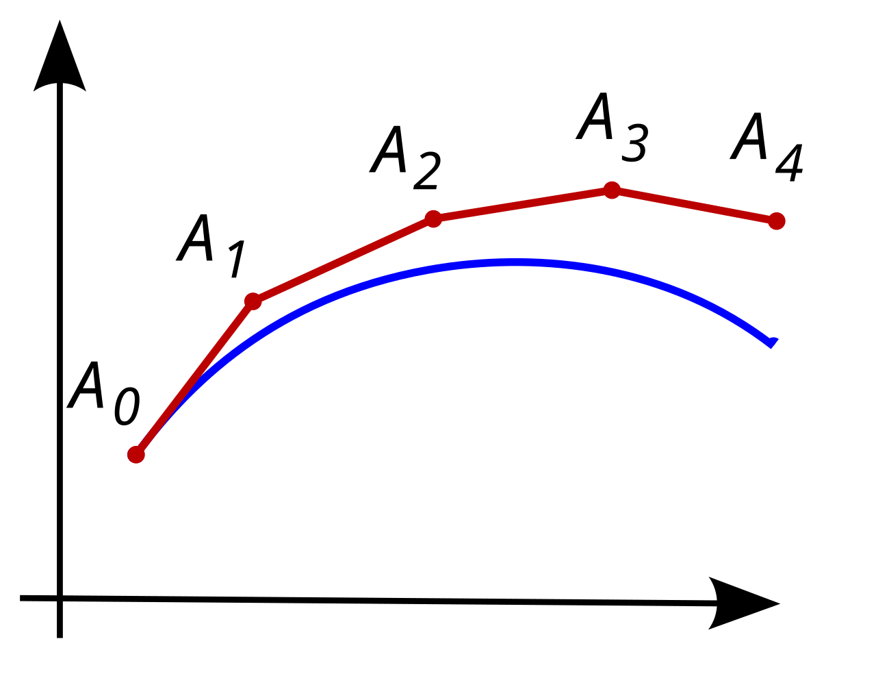
In mathematics and computational science, the Euler method (also called the forward Euler method) is a first-order numerical procedure for solving ordinary differential equations (ODEs) with a given initial value. It is the most basic explicit method for numerical integration of ordinary differential equations and is the simplest Runge–Kutta method. The Euler method is named after Leonhard Euler, who first proposed it in his book Institutionum calculi integralis (published 1768–1770).^[1]

The Euler method is a first-order method, which means that the local error (error per step) is proportional to the square of the step size, and the global error (error at a given time) is proportional to the step size. The Euler method often serves as the basis to construct more complex methods, e.g., predictor–corrector method.

Consider the problem of calculating the shape of an unknown curve which starts at a given point and satisfies a given differential equation. Here, a differential equation can be thought of as a formula by which the slope of the tangent line to the curve can be computed at any point on the curve, once the position of that point has been calculated.

The idea is that while the curve is initially unknown, its starting point, which we denote by ${\displaystyle A_{0},}$ is known (see Figure 1). Then, from the differential equation, the slope to the curve at ${\displaystyle A_{0}}$ can be computed, and so, the tangent line.

Take a small step along that tangent line up to a point ${\displaystyle A_{1}.}$ Along this small step, the slope does not change too much, so ${\displaystyle A_{1}}$ will be close to the curve. If we pretend that ${\displaystyle A_{1}}$ is still on the curve, the same reasoning as for the point ${\displaystyle A_{0}}$ above can be used. After several steps, a polygonal curve (${\displaystyle A_{0}A_{1}A_{2}A_{3}\dots }$) is computed. In general, this curve does not diverge too far from the original unknown curve, and the error between the two curves can be made small if the step size is small enough and the interval of computation is finite.^[2]

When given the values for ${\displaystyle t_{0}}$ and ${\displaystyle y(t_{0})}$, and the derivative of ${\displaystyle y}$ is a given function of ${\displaystyle t}$ and ${\displaystyle y}$ denoted as ${\displaystyle y'(t)=f{\bigl (}t,y(t){\bigr )}}$. Begin the process by setting ${\displaystyle y_{0}=y(t_{0})}$. Next, choose a value ${\displaystyle h}$ for the size of every step along t-axis, and set ${\displaystyle t_{n}=t_{0}+nh}$ (or equivalently ${\displaystyle t_{n+1}=t_n}$