 Hispanopedia Wiki
En ingeniería y ciencia , el análisis dimensional de diferentes magnitudes físicas consiste en el análisis de su dimensión física o dimensión de magnitud , definida como una expresión matemática que identifica las potencias de las magnitudes básicas involucradas (como longitud , masa , tiempo , etc.), y el seguimiento de estas dimensiones a medida que se realizan cálculos o comparaciones. [ 1 ] Los conceptos de análisis dimensional y dimensión de magnitud fueron introducidos por Joseph Fourier en 1822. [ 2 ] : 42
Las magnitudes físicas conmensurables tienen la misma dimensión y son del mismo tipo , por lo que pueden compararse directamente entre sí, incluso si se expresan en unidades de medida diferentes ; por ejemplo, metros y pies, gramos y libras, segundos y años. Las magnitudes físicas inconmensurables tienen dimensiones diferentes, por lo que no pueden compararse directamente entre sí, independientemente de las unidades en las que se expresen; por ejemplo, metros y gramos, segundos y gramos, metros y segundos. Por ejemplo, preguntar si un gramo es mayor que una hora carece de sentido.
Toda ecuación o desigualdad con significado físico debe tener las mismas dimensiones en sus lados izquierdo y derecho, una propiedad conocida como homogeneidad dimensional . La verificación de la homogeneidad dimensional es una aplicación común del análisis dimensional, que sirve como comprobación de plausibilidad para ecuaciones y cálculos derivados . También sirve como guía y restricción para derivar ecuaciones que puedan describir un sistema físico en ausencia de una derivación más rigurosa.
Formulación
El teorema π de Buckingham describe cómo toda ecuación con significado físico que involucre n variables puede reescribirse de forma equivalente como una ecuación con n − m parámetros adimensionales, donde m es el rango de la matriz dimensional . Además, y lo que es más importante, proporciona un método para calcular estos parámetros adimensionales a partir de las variables dadas.
A dimensional equation can have the dimensions reduced or eliminated through nondimensionalization, which begins with dimensional analysis, and involves scaling quantities by characteristic units of a system or physical constants of nature.[2]:43 This may give insight into the fundamental properties of the system, as illustrated in the examples below.
The dimension of a physical quantity can be expressed as a product of the base physical dimensions such as length, mass and time, each raised to an integer (and occasionally rational) power. The dimension of a physical quantity is more fundamental than some scale or unit used to express the amount of that physical quantity. For example, mass is a dimension, while the kilogram is a particular reference quantity chosen to express a quantity of mass. The choice of unit is arbitrary, and its choice is often based on historical precedent. Natural units, being based on only universal constants, may be thought of as being "less arbitrary".
There are many possible choices of base physical dimensions. The SI standard selects the following dimensions and corresponding dimension symbols:
- time (T), length (L), mass (M), electric current (I), absolute temperature (Θ), amount of substance (N) and luminous intensity (J).
The symbols are by convention usually written in romansans serif typeface.[3] Mathematically, the dimension of the quantity Q is given by

where a, b, c, d, e, f, g are the dimensional exponents. Other physical quantities could be defined as the base quantities, as long as they form a basis – for instance, one could replace the dimension (I) of electric current of the SI basis with a dimension (Q) of electric charge, since Q = TI.
A quantity that has only b ≠ 0 (with all other exponents zero) is known as a geometric quantity. A quantity that has only both a ≠ 0 and b ≠ 0 is known as a kinematic quantity. A quantity that has only all of a ≠ 0, b ≠ 0, and c ≠ 0 is known as a dynamic quantity.[4] A quantity that has all exponents null is said to have dimension one.[3]
The unit chosen to express a physical quantity and its dimension are related, but not identical concepts. The units of a physical quantity are defined by convention and related to some standard; e.g., length may have units of metres, feet, inches, miles or micrometres; but any length always has a dimension of L, no matter what units of length are chosen to express it. Two different units of the same physical quantity have conversion factors that relate them. For example, 1 in = 2.54 cm; in this case 2.54 cm/in is the conversion factor, which is itself dimensionless and equal to 1. Therefore, multiplying by that conversion factor does not change either the dimensions nor the value of the physical quantity.
There are also physicists who have cast doubt on the very existence of incompatible fundamental dimensions of physical quantity,[5] although this does not invalidate the usefulness of dimensional analysis.
Simple cases
As examples, the dimension of the physical quantity velocityv is

The dimension of the physical quantity accelerationa is

The dimension of the physical quantity forceF is

The dimension of the physical quantity pressureP is

The dimension of the physical quantity energyE is

The dimension of the physical quantity powerP is

The dimension of the physical quantity electric chargeQ is

The dimension of the physical quantity voltageV is

The dimension of the physical quantity capacitanceC is

Rayleigh's method
En el análisis dimensional, el método de Rayleigh es una herramienta conceptual utilizada en física , química e ingeniería . Expresa la relación funcional de algunas variables mediante una ecuación exponencial . Recibe su nombre de Lord Rayleigh .
El método consta de los siguientes pasos:
- Reúna todas las variables independientes que puedan influir en la variable dependiente .
- Si R es una variable que depende de las variables independientes R 1 , R 2 , R 3 , ..., R n , entonces la ecuación funcional se puede escribir como R = F ( R 1 , R 2 , R 3 , ..., R n ) .
- Escribe la ecuación anterior en la forma R = C R 1 a R 2 b R 3 c ... R n m , donde C es una constante adimensional y a , b , c , ..., m son exponentes arbitrarios.
- Exprese cada una de las cantidades de la ecuación en algunas unidades base en las que se requiere la solución.
- Utilizando la homogeneidad dimensional , obtenga un conjunto de ecuaciones simultáneas que involucren los exponentes a , b , c , ..., m .
- Resuelve estas ecuaciones para obtener los valores de los exponentes a , b , c , ..., m .
- Sustituya los valores de los exponentes en la ecuación principal y forme los parámetros adimensionales agrupando las variables con exponentes iguales.
Como desventaja, el método de Rayleigh no proporciona ninguna información sobre el número de grupos adimensionales que se obtendrán como resultado del análisis dimensional.
Números concretos y unidades básicas
Muchos parámetros y mediciones en las ciencias físicas y la ingeniería se expresan como un número concreto : una cantidad numérica y su correspondiente unidad dimensional. A menudo, una cantidad se expresa en términos de varias otras cantidades; por ejemplo, la velocidad es una combinación de longitud y tiempo, como 60 kilómetros por hora o 1,4 kilómetros por segundo. Las relaciones compuestas con "por" se expresan mediante la división , como 60 km/h. Otras relaciones pueden implicar la multiplicación (que suele representarse con un punto centrado o yuxtaposición ), potencias (como m² para metros cuadrados) o combinaciones de estas.
Un conjunto de unidades base para un sistema de medición es un conjunto de unidades elegido convencionalmente, ninguna de las cuales puede expresarse como una combinación de las demás y en términos de las cuales se pueden expresar todas las unidades restantes del sistema. [ 6 ] Por ejemplo, las unidades de longitud y tiempo se eligen normalmente como unidades base. Sin embargo, las unidades de volumen pueden factorizarse en las unidades base de longitud (m³ ) , por lo que se consideran unidades derivadas o compuestas.
A veces, los nombres de las unidades ocultan el hecho de que son unidades derivadas. Por ejemplo, un newton (N) es una unidad de fuerza , que puede expresarse como el producto de la masa (con unidad kg) y la aceleración (con unidad m⋅s⁻² ) . El newton se define como 1 N = 1 kg⋅m⋅s⁻² .
Porcentajes, derivadas e integrales
Los porcentajes son cantidades adimensionales, ya que son razones de dos cantidades con las mismas dimensiones. En otras palabras, el signo % se puede leer como "centésimas", puesto que 1% = 1/100 .
Al derivar una cantidad, se divide la dimensión por la dimensión de la variable con respecto a la cual se deriva. Por lo tanto:
- La posición ( x ) tiene la dimensión L (longitud);
- La derivada de la posición con respecto al tiempo ( dx / dt , velocidad ) tiene dimensión T −1 L—longitud desde la posición, tiempo debido a la derivada;
- La segunda derivada ( d 2 x / dt 2 = d ( dx / dt ) / dt , aceleración ) tiene dimensión T −2 L .
De igual modo, al tomar una integral se añade la dimensión de la variable con respecto a la cual se está integrando, pero en el numerador.
- La fuerza tiene la dimensión T −2 L M (masa multiplicada por aceleración);
- la integral de fuerza con respecto a la distancia ( s ) que ha recorrido el objeto ( , trabajo ) tiene dimensión T −2 L 2 M .

En economía, se distingue entre existencias y flujos : una existencia tiene una unidad (por ejemplo, productos o dólares), mientras que un flujo es un derivado de una existencia y tiene una unidad de la forma de esta unidad dividida por una unidad de tiempo (por ejemplo, dólares/año).
En algunos contextos, las cantidades dimensionales se expresan como cantidades adimensionales o porcentajes omitiendo algunas dimensiones. Por ejemplo, los ratios deuda/PIB se suelen expresar como porcentajes: deuda total pendiente (dimensión monetaria) dividida por el PIB anual (dimensión monetaria). Sin embargo, se podría argumentar que, al comparar un stock con un flujo, el PIB anual debería tener dimensiones monetarias/temporales (dólares/año, por ejemplo) y, por lo tanto, la relación deuda/PIB debería tener la unidad anual, lo que indica que esta relación representa el número de años necesarios para que un PIB constante pague la deuda, si todo el PIB se destina al pago de la deuda y esta permanece invariable.
Homogeneidad dimensional (conmensurabilidad)
La regla más básica del análisis dimensional es la de homogeneidad dimensional. [ 7 ]
Sin embargo, las dimensiones forman un grupo abeliano bajo la multiplicación, por lo que:
Por ejemplo, no tiene sentido preguntar si 1 hora es más, lo mismo o menos que 1 kilómetro, ya que tienen dimensiones diferentes, ni tampoco sumar 1 hora a 1 kilómetro. Sin embargo, sí tiene sentido preguntar si 1 milla es más, lo mismo o menos que 1 kilómetro, pues se trata de la misma magnitud física aunque las unidades sean diferentes. Por otro lado, si un objeto recorre 100 km en 2 horas, se puede dividir este tiempo y concluir que su velocidad media fue de 50 km/h.
La regla implica que, en una expresión físicamente significativa , solo se pueden sumar, restar o comparar cantidades de la misma dimensión. Por ejemplo, si m hombre , m rata y L hombre denotan, respectivamente, la masa de un hombre, la masa de una rata y la longitud de ese hombre, la expresión dimensionalmente homogénea m hombre + m rata tiene sentido, pero la expresión heterogénea m hombre + L hombre carece de sentido. Sin embargo, m hombre / L² hombre es válida. Por lo tanto, el análisis dimensional puede utilizarse como una comprobación de coherencia de las ecuaciones físicas: ambos lados de cualquier ecuación deben ser conmensurables o tener las mismas dimensiones.
Incluso cuando dos magnitudes físicas tienen dimensiones idénticas, compararlas o sumarlas puede resultar inútil. Por ejemplo, aunque el par motor y la energía comparten la dimensión T −2 L 2 M , son magnitudes físicas fundamentalmente diferentes.
Para comparar, sumar o restar cantidades con las mismas dimensiones pero expresadas en unidades diferentes, el procedimiento estándar consiste en convertirlas primero a la misma unidad. Por ejemplo, para comparar 32 metros con 35 yardas, se utiliza la equivalencia 1 yarda = 0,9144 m para convertir 35 yardas a 32,004 m.
Un principio relacionado es que cualquier ley física que describa con precisión el mundo real debe ser independiente de las unidades utilizadas para medir las variables físicas. [ 8 ] Por ejemplo, las leyes del movimiento de Newton deben ser válidas tanto si la distancia se mide en millas como en kilómetros. Este principio da lugar a la fórmula de que un factor de conversión entre dos unidades que miden la misma dimensión debe ser el producto de una constante simple. También garantiza la equivalencia; por ejemplo, si dos edificios tienen la misma altura en pies, entonces deben tener la misma altura en metros.
Por ejemplo, si se calcula una velocidad , las unidades siempre deben combinarse como L/T; si se calcula una energía , las unidades siempre deben combinarse como ML² / T² , etc. Por ejemplo, las siguientes fórmulas podrían ser expresiones válidas para alguna energía:

Si m es una masa, v y c son velocidades , p es un momento , h es la constante de Planck , λ una longitud. Por otro lado, si las unidades del lado derecho no se combinan para dar [masa][longitud] ² /[tiempo] ² , no puede ser una expresión válida para alguna energía .
Ser homogéneo no significa necesariamente que la ecuación sea verdadera, ya que no tiene en cuenta factores numéricos. Por ejemplo, E = mv² podría ser o no ser la fórmula correcta para la energía de una partícula de masa m que viaja a velocidad v , y no se puede saber si hc / λ debe dividirse o multiplicarse por 2π .
Factor de conversión
En el análisis dimensional, un cociente que convierte una unidad de medida en otra sin cambiar la magnitud se llama factor de conversión . Por ejemplo, kPa y bar son unidades de presión, y 100 kPa = 1 bar . Las reglas del álgebra permiten dividir ambos lados de una ecuación por la misma expresión, por lo que esto es equivalente a 100 kPa / 1 bar = 1. Dado que cualquier magnitud se puede multiplicar por 1 sin cambiarla, la expresión " 100 kPa / 1 bar " se puede usar para convertir de bares a kPa multiplicándola por la magnitud que se va a convertir, incluyendo la unidad. Por ejemplo, 5 bar × 100 kPa / 1 bar = 500 kPa porque 5 × 100 / 1 = 500 , y bar/bar se cancela, por lo que 5 bar = 500 kPa .
Aplicaciones
El análisis dimensional se utiliza con mayor frecuencia en física y química, y en sus ramas matemáticas, pero también encuentra algunas aplicaciones fuera de esos campos.
Matemáticas
Una aplicación sencilla del análisis dimensional a las matemáticas consiste en calcular la forma del volumen de una n -bola (la esfera sólida en n dimensiones) o el área de su superficie, la n -esfera : al ser una figura n -dimensional, el volumen escala como x n , mientras que el área de la superficie, al ser ( n -1) -dimensional, escala como x n -1 . Así, el volumen de la n -bola en función del radio es C n r n , para alguna constante C n . Determinar la constante requiere matemáticas más complejas, pero la forma puede deducirse y comprobarse únicamente mediante el análisis dimensional.
Finanzas, economía y contabilidad
En finanzas, economía y contabilidad, el análisis dimensional se suele entender como la distinción entre existencias y flujos . En términos más generales, el análisis dimensional se utiliza para interpretar diversos ratios financieros , económicos y contables.
- Por ejemplo, la relación precio/beneficio (P/E) tiene dimensiones de tiempo (unidad: año) y puede interpretarse como "años de ganancias para obtener el precio pagado".
- En economía, la relación deuda/PIB también se expresa en años (la deuda se mide en unidades monetarias, el PIB en unidades monetarias/año).
- La velocidad del dinero tiene una unidad de 1/año (PIB/oferta monetaria tiene una unidad de moneda/año sobre moneda): con qué frecuencia circula una unidad monetaria por año.
- Los tipos de interés anuales con capitalización continua y los tipos de interés simples suelen expresarse como un porcentaje (cantidad adimensional), mientras que el tiempo se expresa como una cantidad adimensional que consiste en el número de años. Sin embargo, si el tiempo incluye el año como unidad de medida, la dimensión del tipo es 1/año. Por supuesto, no hay nada especial (aparte de la convención habitual) en usar el año como unidad de tiempo: se puede usar cualquier otra unidad de tiempo. Además, si el tipo y el tiempo incluyen sus unidades de medida, el uso de unidades diferentes para cada uno no supone ningún problema. En cambio, si el tipo y el tiempo son adimensionales, deben referirse a un período común. (Cabe señalar que los tipos de interés efectivos solo pueden definirse como cantidades adimensionales).
- In financial analysis, bond duration can be defined as (dV/dr)/V, where V is the value of a bond (or portfolio), r is the continuously compounded interest rate and dV/dr is a derivative. From the previous point, the dimension of r is 1/time. Therefore, the dimension of duration is time (usually expressed in years) because dr is in the "denominator" of the derivative.
Fluid mechanics
In fluid mechanics, dimensional analysis is performed to obtain dimensionless pi terms or groups. According to the principles of dimensional analysis, any prototype can be described by a series of these terms or groups that describe the behaviour of the system. Using suitable pi terms or groups, it is possible to develop a similar set of pi terms for a model that has the same dimensional relationships.[9] In other words, pi terms provide a shortcut to developing a model representing a certain prototype. Common dimensionless groups in fluid mechanics include:
- Reynolds number (Re), generally important in all types of fluid problems:
- Froude number (Fr), modeling flow with a free surface:
- Euler number (Eu), used in problems in which pressure is of interest:
- Mach number (Ma), important in high speed flows where the velocity approaches or exceeds the local speed of sound: where c is the local speed of sound.


History
The origins of dimensional analysis have been disputed by historians.[10][11] The first written application of dimensional analysis has been credited to François Daviet, a student of Joseph-Louis Lagrange, in a 1799 article at the Turin Academy of Science.[11]
This led to the conclusion that meaningful laws must be homogeneous equations in their various units of measurement, a result which was eventually later formalized in the Buckingham π theorem. Simeon Poisson also treated the same problem of the parallelogram law by Daviet, in his treatise of 1811 and 1833 (vol I, p. 39).[12] In the second edition of 1833, Poisson explicitly introduces the term dimension instead of the Daviet homogeneity.
In 1822, the important Napoleonic scientist Joseph Fourier made the first credited important contributions[13] based on the idea that physical laws like F = ma should be independent of the units employed to measure the physical variables.
James Clerk Maxwell and Fleeming Jenkin played a major role in establishing modern use of dimensional analysis by distinguishing mass, length, and time as fundamental units, while referring to other units as derived.[14][15] Although Maxwell defined length, time and mass to be "the three fundamental units", he also noted that gravitational mass can be derived from length and time by assuming a form of Newton's law of universal gravitation in which the gravitational constantG is taken as unity, thereby defining M = T−2L3.[16] By assuming a form of Coulomb's law in which the Coulomb constantke is taken as unity, Maxwell then determined that the dimensions of an electrostatic unit of charge were Q = T−1L3/2M1/2,[17] which, after substituting his M = T−2L3 equation for mass, results in charge having the same dimensions as mass, viz. Q = T−2L3.
Dimensional analysis is also used to derive relationships between the physical quantities that are involved in a particular phenomenon that one wishes to understand and characterize. It was used for the first time in this way in 1872 by Lord Rayleigh, who was trying to understand why the sky is blue.[18] Rayleigh first published the technique in his 1877 book The Theory of Sound.[19]
The original meaning of the word dimension, in Fourier's Theorie de la Chaleur, was the numerical value of the exponents of the base units. For example, acceleration was considered to have the dimension 1 with respect to the unit of length, and the dimension −2 with respect to the unit of time.[20] This was slightly changed by Maxwell, who said the dimensions of acceleration are T−2L, instead of just the exponents.[21]
Examples
A simple example: period of a harmonic oscillator
What is the period of oscillationT of a mass m attached to an ideal linear spring with spring constant k suspended in gravity of strength g? That period is the solution for T of some dimensionless equation in the variables T, m, k, and g. The four quantities have the following dimensions: T (T); m (M); k (M/T2); and g (L/T2). From these we can form only one dimensionless product of powers of our chosen variables, G1 = T2k/m(T2 · M/T2 / M = 1), and putting G1 = C for some dimensionless constant C gives the dimensionless equation sought. The dimensionless product of powers of variables is sometimes referred to as a dimensionless group of variables; here the term "group" means "collection" rather than mathematical group. They are often called dimensionless numbers as well.
The variable g does not occur in the group. It is easy to see that it is impossible to form a dimensionless product of powers that combines g with k, m, and T, because g is the only quantity that involves the dimension L. This implies that in this problem the g is irrelevant. Dimensional analysis can sometimes yield strong statements about the irrelevance of some quantities in a problem, or the need for additional parameters. If we have chosen enough variables to properly describe the problem, then from this argument we can conclude that the period of the mass on the spring is independent of g: it is the same on the earth or the moon. The equation demonstrating the existence of a product of powers for our problem can be written in an entirely equivalent way: , for some dimensionless constant κ (equal to from the original dimensionless equation).


When faced with a case where dimensional analysis rejects a variable (g, here) that one intuitively expects to belong in a physical description of the situation, another possibility is that the rejected variable is in fact relevant, but that some other relevant variable has been omitted, which might combine with the rejected variable to form a dimensionless quantity. That is, however, not the case here.
When dimensional analysis yields only one dimensionless group, as here, there are no unknown functions, and the solution is said to be "complete" – although it still may involve unknown dimensionless constants, such as κ.
A more complex example: energy of a vibrating wire
Consider the case of a vibrating wire of lengthℓ (L) vibrating with an amplitudeA (L). The wire has a linear densityρ (M/L) and is under tensions (LM/T2), and we want to know the energy E (L2M/T2) in the wire. Let π1 and π2 be two dimensionless products of powers of the variables chosen, given by

The linear density of the wire is not involved. The two groups found can be combined into an equivalent form as an equation
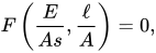
where F is some unknown function, or, equivalently as
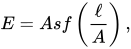
where f is some other unknown function. Here the unknown function implies that our solution is now incomplete, but dimensional analysis has given us something that may not have been obvious: the energy is proportional to the first power of the tension. Barring further analytical analysis, we might proceed to experiments to discover the form for the unknown function f. But our experiments are simpler than in the absence of dimensional analysis. We'd perform none to verify that the energy is proportional to the tension. Or perhaps we might guess that the energy is proportional to ℓ, and so infer that E = ℓs. The power of dimensional analysis as an aid to experiment and forming hypotheses becomes evident.
El poder del análisis dimensional se hace realmente evidente cuando se aplica a situaciones, distintas a las mencionadas anteriormente, que son más complejas, donde el conjunto de variables involucradas no es evidente y las ecuaciones subyacentes son sumamente complejas. Consideremos, por ejemplo, una pequeña piedra sobre el lecho de un río. Si el río fluye con la suficiente rapidez, la piedra se elevará y será arrastrada por la corriente. ¿A qué velocidad crítica ocurrirá esto? Determinar las variables supuestas no es tan sencillo como antes. Sin embargo, el análisis dimensional puede ser una herramienta poderosa para comprender problemas como este, y suele ser la primera que se aplica a problemas complejos donde las ecuaciones y restricciones subyacentes no se comprenden bien. En tales casos, la respuesta puede depender de un número adimensional , como el número de Reynolds , que puede interpretarse mediante el análisis dimensional.
Un tercer ejemplo: demanda frente a capacidad para un disco giratorio.

Consideremos el caso de un disco delgado, sólido, de caras paralelas y giratorio, con un espesor axial t (L) y un radio R ( L). El disco tiene una densidad ρ (M/L³ ) , gira a una velocidad angular ω (T⁻¹ ) y esto produce una tensión S (T⁻²L⁻¹M ) en el material. Existe una solución elástica lineal teórica, propuesta por Lamé, para este problema cuando el disco es delgado en relación con su radio, las caras del disco pueden moverse axialmente libremente y se pueden asumir las relaciones constitutivas de tensión plana. A medida que el disco se vuelve más grueso en relación con el radio, la solución de tensión plana deja de ser válida. Si el disco está restringido axialmente en sus caras libres, se producirá un estado de deformación plana. Sin embargo, si este no es el caso, el estado de tensión solo puede determinarse mediante la consideración de la elasticidad tridimensional y no existe una solución teórica conocida para este caso. Por lo tanto, un ingeniero podría estar interesado en establecer una relación entre las cinco variables. El análisis dimensional para este caso conduce a los siguientes grupos adimensionales ( 5 − 3 = 2 ):
- demanda/capacidad = ρR 2 ω 2 / S
- espesor/radio o relación de aspecto = t / R
Mediante experimentos numéricos, utilizando, por ejemplo, el método de elementos finitos , se puede obtener la naturaleza de la relación entre los dos grupos adimensionales, como se muestra en la figura. Dado que este problema solo involucra dos grupos adimensionales, se proporciona una imagen completa en un solo gráfico, que puede utilizarse como diagrama de diseño/evaluación para discos giratorios. [ 22 ]
Propiedades
Propiedades matemáticas
Las dimensiones que se pueden formar a partir de un conjunto dado de dimensiones físicas básicas, como T, L y M, forman un grupo abeliano : la identidad se escribe como 1; L 0 = 1 , y el inverso de L es 1/L o L −1 . L elevado a cualquier potencia entera p es un miembro del grupo, teniendo un inverso de L − p o 1/L p . La operación del grupo es la multiplicación, con las reglas habituales para manejar exponentes ( L n × L m = L n + m ). Físicamente, 1/L puede interpretarse como longitud recíproca , y 1/T como tiempo recíproco (véase segundo recíproco ).
Un grupo abeliano es equivalente a un módulo sobre los enteros, donde el símbolo dimensional T i L j M k corresponde a la tupla ( i , j , k ) . Cuando cantidades físicas medidas (ya sean de la misma dimensión o de dimensiones diferentes) se multiplican o dividen entre sí, sus unidades dimensionales también se multiplican o dividen; esto corresponde a la suma o resta en el módulo. Cuando cantidades medibles se elevan a una potencia entera, se realiza la misma operación con los símbolos dimensionales asociados a dichas cantidades; esto corresponde a la multiplicación escalar en el módulo.
La base de un módulo de símbolos dimensionales se denomina conjunto de cantidades base , y todos los demás vectores se denominan unidades derivadas. Como en cualquier módulo, se pueden elegir diferentes bases , lo que da lugar a diferentes sistemas de unidades (por ejemplo, elegir si la unidad de carga se deriva de la unidad de corriente, o viceversa).
La identidad del grupo, la dimensión de cantidades adimensionales, corresponde al origen en este módulo, (0, 0, 0) .
En ciertos casos, se pueden definir dimensiones fraccionarias, específicamente definiendo formalmente potencias fraccionarias de espacios vectoriales unidimensionales, como V L 1/2 . [ 23 ] Sin embargo, no es posible tomar potencias fraccionarias arbitrarias de unidades, debido a obstrucciones de la teoría de la representación . [ 24 ]
Se puede trabajar con espacios vectoriales de dimensiones dadas sin necesidad de usar unidades (que corresponden a los sistemas de coordenadas de los espacios vectoriales). Por ejemplo, dadas las dimensiones M y L , se tienen los espacios vectoriales V M y V L , y se puede definir V ML := V M ⊗ V L como el producto tensorial . De manera similar, el espacio dual puede interpretarse como si tuviera dimensiones "negativas". [ 25 ] Esto corresponde al hecho de que, bajo el emparejamiento natural entre un espacio vectorial y su dual, las dimensiones se cancelan, dejando un escalar adimensional .
El conjunto de unidades de las magnitudes físicas involucradas en un problema corresponde a un conjunto de vectores (o una matriz). La nulidad describe un número (por ejemplo, m ) de maneras en que estos vectores pueden combinarse para producir un vector cero. Esto corresponde a producir (a partir de las mediciones) una serie de magnitudes adimensionales, {π 1 , ..., π m } . (De hecho, estas maneras abarcan completamente el subespacio nulo de otro espacio diferente, el de las potencias de las mediciones). Cada forma posible de multiplicar (y exponenciar ) las magnitudes medidas para producir algo con la misma unidad que alguna magnitud derivada X puede expresarse en la forma general
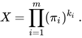
En consecuencia, toda ecuación conmensurable posible para la física del sistema puede reescribirse en la forma

Conocer esta restricción puede ser una herramienta poderosa para obtener nuevos conocimientos sobre el sistema.
Mecánica
The dimension of physical quantities of interest in mechanics can be expressed in terms of base dimensions T, L, and M – these form a 3-dimensional vector space. This is not the only valid choice of base dimensions, but it is the one most commonly used. For example, one might choose force, length and mass as the base dimensions (as some have done), with associated dimensions F, L, M; this corresponds to a different basis, and one may convert between these representations by a change of basis. The choice of the base set of dimensions is thus a convention, with the benefit of increased utility and familiarity. The choice of base dimensions is not entirely arbitrary, because they must form a basis: they must span the space, and be linearly independent.
For example, F, L, M form a set of fundamental dimensions because they form a basis that is equivalent to T, L, M: the former can be expressed as [F = LM/T2], L, M, while the latter can be expressed as [T = (LM/F)1/2], L, M.
On the other hand, length, velocity and time (T, L, V) do not form a set of base dimensions for mechanics, for two reasons:
- There is no way to obtain mass – or anything derived from it, such as force – without introducing another base dimension (thus, they do not span the space).
- Velocity, being expressible in terms of length and time (V = L/T), is redundant (the set is not linearly independent).
Other fields of physics and chemistry
Depending on the field of physics, it may be advantageous to choose one or another extended set of dimensional symbols. In electromagnetism, for example, it may be useful to use dimensions of T, L, M and Q, where Q represents the dimension of electric charge. In thermodynamics, the base set of dimensions is often extended to include a dimension for temperature, Θ. In chemistry, the amount of substance (the number of molecules divided by the Avogadro constant, ≈ 6.02×10²³ mol−1) is also defined as a base dimension, N. In the interaction of relativistic plasma with strong laser pulses, a dimensionless relativistic similarity parameter, connected with the symmetry properties of the collisionless Vlasov equation, is constructed from the plasma-, electron- and critical-densities in addition to the electromagnetic vector potential. The choice of the dimensions or even the number of dimensions to be used in different fields of physics is to some extent arbitrary, but consistency in use and ease of communications are common and necessary features.
Polynomials and transcendental functions
Bridgman's theorem restricts the type of function that can be used to define a physical quantity from general (dimensionally compounded) quantities to only products of powers of the quantities, unless some of the independent quantities are algebraically combined to yield dimensionless groups, whose functions are grouped together in the dimensionless numeric multiplying factor.[26][27] This excludes polynomials of more than one term or transcendental functions not of that form.
Scalar arguments to transcendental functions such as exponential, trigonometric and logarithmic functions, or to inhomogeneous polynomials, must be dimensionless quantities. (Note: this requirement is somewhat relaxed in Siano's orientational analysis described below, in which the square of certain dimensioned quantities are dimensionless.)
While most mathematical identities about dimensionless numbers translate in a straightforward manner to dimensional quantities, care must be taken with logarithms of ratios: the identity log(a/b) = loga − logb, where the logarithm is taken in any base, holds for dimensionless numbers a and b, but it does not hold if a and b are dimensional, because in this case the left-hand side is well-defined but the right-hand side is not.[28]
Similarly, while one can evaluate monomials (xn) of dimensional quantities, one cannot evaluate polynomials of mixed degree with dimensionless coefficients on dimensional quantities: for x2, the expression (3 m)2 = 9 m2 makes sense (as an area), while for x2 + x, the expression (3 m)2 + 3 m = 9 m2 + 3 m does not make sense.
However, polynomials of mixed degree can make sense if the coefficients are suitably chosen physical quantities that are not dimensionless. For example,

This is the height to which an object rises in time t if the acceleration of gravity is 9.8 metres per second per second and the initial upward speed is 500 metres per second. It is not necessary for t to be in seconds. For example, suppose t = 0.01 minutes. Then the first term would be
![{\displaystyle {\begin{aligned}&{\tfrac {1}{2}}\cdot (\mathrm {-9.8~m/s^{2}} )\cdot (\mathrm {0.01~min} )^{2}\\[10pt]={}&{\tfrac {1}{2}}\cdot -9.8\cdot \left(0.01^{2}\right)(\mathrm {min/s} )^{2}\cdot \mathrm {m} \\[10pt]={}&{\tfrac {1}{2}}\cdot -9.8\cdot \left(0.01^{2}\right)\cdot 60^{2}\cdot \mathrm {m} .\end{aligned}}}](https://wikimedia.org/api/rest_v1/media/math/render/svg/69b5bd672290410cfcc7876ecb6d84b36b7b2421)
Combining units and numerical values
The value of a dimensional physical quantity Z is written as the product of a unit [Z] within the dimension and a dimensionless numerical value or numerical factor, n.[29]
![{\displaystyle Z=n\times [Z]=n[Z]}](https://wikimedia.org/api/rest_v1/media/math/render/svg/a301c02a2b018e24efb3c614727ead393565b8b3)
When like-dimensioned quantities are added or subtracted or compared, it is convenient to express them in the same unit so that the numerical values of these quantities may be directly added or subtracted. But, in concept, there is no problem adding quantities of the same dimension expressed in different units. For example, 1 metre added to 1 foot is a length, but one cannot derive that length by simply adding 1 and 1. A conversion factor, which is a ratio of like-dimensioned quantities and is equal to the dimensionless unity, is needed:
- is identical to

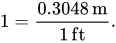
The factor 0.3048 m/ft is identical to the dimensionless 1, so multiplying by this conversion factor changes nothing. Then when adding two quantities of like dimension, but expressed in different units, the appropriate conversion factor, which is essentially the dimensionless 1, is used to convert the quantities to the same unit so that their numerical values can be added or subtracted.
Only in this manner is it meaningful to speak of adding like-dimensioned quantities of differing units.
Quantity equations
A quantity equation, also sometimes called a complete equation, is an equation that remains valid independently of the unit of measurement used when expressing the physical quantities.[30]
In contrast, in a numerical-value equation, just the numerical values of the quantities occur, without units. Therefore, it is only valid when each numerical values is referenced to a specific unit.
For example, a quantity equation for displacementd as speeds multiplied by time difference t would be:
- d = st
for s = 5 m/s, where t and d may be expressed in any units, converted if necessary. In contrast, a corresponding numerical-value equation would be:
- D = 5 T
where T is the numeric value of t when expressed in seconds and D is the numeric value of d when expressed in metres.
Generally, the use of numerical-value equations is discouraged.[30]
Dimensionless concepts
Constants
The dimensionless constants that arise in the results obtained, such as the C in the Poiseuille's Law problem and the κ in the spring problems discussed above, come from a more detailed analysis of the underlying physics and often arise from integrating some differential equation. Dimensional analysis itself has little to say about these constants, but it is useful to know that they very often have a magnitude of order unity. This observation can allow one to sometimes make "back of the envelope" calculations about the phenomenon of interest, and therefore be able to more efficiently design experiments to measure it, or to judge whether it is important, etc.
Formalisms
Paradoxically, dimensional analysis can be a useful tool even if all the parameters in the underlying theory are dimensionless, e.g., lattice models such as the Ising model can be used to study phase transitions and critical phenomena. Such models can be formulated in a purely dimensionless way. As we approach the critical point closer and closer, the distance over which the variables in the lattice model are correlated (the so-called correlation length, χ) becomes larger and larger. Now, the correlation length is the relevant length scale related to critical phenomena, so one can, e.g., surmise on "dimensional grounds" that the non-analytical part of the free energy per lattice site should be ~ 1/χd, where d is the dimension of the lattice.
It has been argued by some physicists, e.g., Michael J. Duff,[5][31] that the laws of physics are inherently dimensionless. The fact that we have assigned incompatible dimensions to Length, Time and Mass is, according to this point of view, just a matter of convention, borne out of the fact that before the advent of modern physics, there was no way to relate mass, length, and time to each other. The three independent dimensionful constants: c, ħ, and G, in the fundamental equations of physics must then be seen as mere conversion factors to convert Mass, Time and Length into each other.
Just as in the case of critical properties of lattice models, one can recover the results of dimensional analysis in the appropriate scaling limit; e.g., dimensional analysis in mechanics can be derived by reinserting the constants ħ, c, and G (but we can now consider them to be dimensionless) and demanding that a nonsingular relation between quantities exists in the limit c → ∞, ħ → 0 and G → 0. In problems involving a gravitational field the latter limit should be taken such that the field stays finite.
Dimensional equivalences
Following are tables of commonly occurring expressions in physics, related to the dimensions of energy, momentum, and force.[32][33][34]
Lenguajes de programación
Dimensional correctness as part of type checking has been studied since 1977.[35] Implementations for Ada[36] and C++[37] were described in 1985 and 1988. Kennedy's 1996 thesis describes an implementation in Standard ML,[38] and later in F#.[39] There are implementations for Haskell,[40]OCaml,[41] and Rust,[42] Python,[43] and a code checker for Fortran.[44][45] Griffioen's 2019 thesis extended Kennedy's Hindley–Milner type system to support Hart's matrices.[46][47] McBride and Nordvall-Forsberg show how to use dependent types to extend type systems for units of measure.[48]
Mathematica 13.2 has a function for transformations with quantities named NondimensionalizationTransform that applies a nondimensionalization transform to an equation.[49] Mathematica also has a function to find the dimensions of a unit such as 1 J named UnitDimensions.[50] Mathematica also has a function that will find dimensionally equivalent combinations of a subset of physical quantities named DimensionalCombinations.[51] Mathematica can also factor out certain dimension with UnitDimensions by specifying an argument to the function UnityDimensions.[52] For example, you can use UnityDimensions to factor out angles.[52] In addition to UnitDimensions, Mathematica can find the dimensions of a QuantityVariable with the function QuantityVariableDimensions.[53]
Geometry: position vs. displacement
Affine quantities
Some discussions of dimensional analysis implicitly describe all quantities as mathematical vectors, but this is not the case. Numbers are often used to represent things that are not elements of vector spaces, and dimensional analysis should not be applied to such things. In physics, scalars are positive quantities like weight or distance with magnitude but not direction (though many authors loosely allow scalars to be negative), vectors can be added to or subtracted from other vectors, and, inter alia, multiplied or divided by scalars. If a vector is used to define a position, this assumes an implicit point of reference: an origin. While this is useful and often perfectly adequate, allowing many important errors to be caught, it can fail to model certain aspects of physics. A more rigorous approach requires distinguishing position from displacement, date from duration, bearing from angle, and absolute temperature from temperature change.
Consider points on a timeline, each with a date with respect to a given origin, and durations of between them. The dates themselves are labels of points, while the durations of time between points have a dimension of time:
- adding two durations should yield a new duration (waiting ten days then twenty days gets you thirty days forward),
- adding a duration to a date should yield a new date (Waiting one month from March 1st, 1900 take you to April 1st.),
- subtracting two dates should yield a duration,
- but one may not add two dates (Adding March 1st to April 1st does not make sense.)
This illustrates the subtle type-distinction between affine values (elements of an affine space, such as date) and vector values (elements of a vector space, such as duration).
- Vectors may be added to each other, yielding a new vector, and a vector may be added to a suitable affine quantity (a vector space acts on an affine space), yielding a new affine quantity.
- Affine quantities cannot be added, but may be subtracted, yielding relative quantities which are vectors, and these relative differences may then be added to each other or to an affine quantity.
Properly then dates and positions are not dimensional quantities but affine quantities. Durations and displacements are dimensional quantities. To represent dimensional quantities with numbers, one must only select a reference unit. To represent affine quantities like date and position in terms of dimensional quantity, one must also select a point of reference and coordinate system in addition to the reference unit.
While some quantities are well-represented by vector quantities to which dimensional analysis can be applied, others are more naturally represented in an affine space, and still others like bearings and probabilities are elements of other spaces.
This distinction is particularly important in the case of temperature, for which the numeric value of absolute zero is not the origin 0 in some scales. For absolute zero,
- −273.15 °C ≘ 0 K = 0 °R ≘ −459.67 °F,
where the symbol ≘ means corresponds to, since although these values on the respective temperature scales correspond, they represent distinct quantities in the same way that the distances from distinct starting points to the same end point are distinct quantities, and cannot in general be equated.
For temperature differences,
- 1 K = 1 °C ≠ 1 °F = 1 °R.
(Here °R refers to the Rankine scale, not the Réaumur scale). Unit conversion for temperature differences is simply a matter of multiplying by, e.g., 1 °F / 1 K. But because some of these scales have origins that do not correspond to absolute zero, conversion from one temperature scale to another requires accounting for that. As a result, simple dimensional analysis can lead to errors if it is ambiguous whether 1 K means the absolute temperature corresponding to the Celsius temperature −272.15 °C, or a temperature difference equal to 1 °C.
Orientation and frame of reference
Similar to the issue of a point of reference is the issue of orientation: a displacement in 2 or 3 dimensions is not just a length, but is a length together with a direction. (In 1 dimension, this issue is equivalent to the distinction between positive and negative.) Thus, to compare or combine two dimensional quantities in multi-dimensional Euclidean space, one also needs a bearing: they need to be compared to a frame of reference.
This leads to the extensions discussed below, namely Huntley's directed dimensions and Siano's orientational analysis.
Huntley's extensions
Huntley has pointed out that a dimensional analysis can become more powerful by discovering new independent dimensions in the quantities under consideration, thus increasing the rank of the dimensional matrix.[54]

He introduced two approaches:
- The magnitudes of the components of a vector are to be considered dimensionally independent. For example, rather than an undifferentiated length dimension L, we may have Lx represent dimension in the x-direction, and so forth. This requirement stems ultimately from the requirement that each component of a physically meaningful equation (scalar, vector, or tensor) must be dimensionally consistent.
- Mass as a measure of the quantity of matter is to be considered dimensionally independent from mass as a measure of inertia.
Directed dimensions
As an example of the usefulness of the first approach, suppose we wish to calculate the distance a cannonball travels when fired with a vertical velocity component and a horizontal velocity component , assuming it is fired on a flat surface. Assuming no use of directed lengths, the quantities of interest are then R, the distance travelled, with dimension L, , , both dimensioned as T−1L, and g the downward acceleration of gravity, with dimension T−2L.


With these four quantities, we may conclude that the equation for the range R may be written:
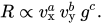
Or dimensionally

from which we may deduce that and , which leaves one exponent undetermined. This is to be expected since we have two fundamental dimensions T and L, and four parameters, with one equation.


However, if we use directed length dimensions, then will be dimensioned as T−1Lx, as T−1Ly, R as Lx and g as T−2Ly. The dimensional equation becomes:



and we may solve completely as a = 1, b = 1 and c = −1. The increase in deductive power gained by the use of directed length dimensions is apparent.
Huntley's concept of directed length dimensions however has some serious limitations:
- It does not deal well with vector equations involving the cross product,
- nor does it handle well the use of angles as physical variables.
It also is often quite difficult to assign the L, Lx, Ly, Lz, symbols to the physical variables involved in the problem of interest. He invokes a procedure that involves the "symmetry" of the physical problem. This is often very difficult to apply reliably: It is unclear as to what parts of the problem that the notion of "symmetry" is being invoked. Is it the symmetry of the physical body that forces are acting upon, or to the points, lines or areas at which forces are being applied? What if more than one body is involved with different symmetries?
Consider the spherical bubble attached to a cylindrical tube, where one wants the flow rate of air as a function of the pressure difference in the two parts. What are the Huntley extended dimensions of the viscosity of the air contained in the connected parts? What are the extended dimensions of the pressure of the two parts? Are they the same or different? These difficulties are responsible for the limited application of Huntley's directed length dimensions to real problems.
Quantity of matter
In Huntley's second approach, he holds that it is sometimes useful (e.g., in fluid mechanics and thermodynamics) to distinguish between mass as a measure of inertia (inertial mass), and mass as a measure of the quantity of matter. Quantity of matter is defined by Huntley as a quantity only proportional to inertial mass, while not implicating inertial properties. No further restrictions are added to its definition.
For example, consider the derivation of Poiseuille's Law. We wish to find the rate of mass flow of a viscous fluid through a circular pipe. Without drawing distinctions between inertial and substantial mass, we may choose as the relevant variables:
There are three fundamental variables, so the above five equations will yield two independent dimensionless variables:


If we distinguish between inertial mass with dimension and quantity of matter with dimension , then mass flow rate and density will use quantity of matter as the mass parameter, while the pressure gradient and coefficient of viscosity will use inertial mass. We now have four fundamental parameters, and one dimensionless constant, so that the dimensional equation may be written:


where now only C is an undetermined constant (found to be equal to by methods outside of dimensional analysis). This equation may be solved for the mass flow rate to yield Poiseuille's law.

Huntley's recognition of quantity of matter as an independent quantity dimension is evidently successful in the problems where it is applicable, but his definition of quantity of matter is open to interpretation, as it lacks specificity beyond the two requirements he postulated for it. For a given substance, the SI dimension amount of substance, with unit mole, does satisfy Huntley's two requirements as a measure of quantity of matter, and could be used as a quantity of matter in any problem of dimensional analysis where Huntley's concept is applicable.
Siano's extension: orientational analysis
Angles are, by convention, considered to be dimensionless quantities (although the wisdom of this is contested).[55] As an example, consider again the projectile problem in which a point mass is launched from the origin (x, y) = (0, 0) at a speed v and angle θ above the x-axis, with the force of gravity directed along the negative y-axis. It is desired to find the range R, at which point the mass returns to the x-axis. Conventional analysis will yield the dimensionless variable π = Rg/v2, but offers no insight into the relationship between R and θ.
Siano has suggested that the directed dimensions of Huntley be replaced by using orientational symbols1x 1y 1z to denote vector directions, and an orientationless symbol 10.[56] Thus, Huntley's Lx becomes L1x with L specifying the dimension of length, and 1x specifying the orientation. Siano further shows that the orientational symbols have an algebra of their own. Along with the requirement that 1i−1 = 1i, the following multiplication table for the orientation symbols results:
The orientational symbols form a group (the Klein four-group or "Viergruppe"). In this system, scalars always have the same orientation as the identity element, independent of the "symmetry of the problem". Physical quantities that are vectors have the orientation expected: a force or a velocity in the z-direction has the orientation of 1z. For angles, consider an angle θ that lies in the z-plane. Form a right triangle in the z-plane with θ being one of the acute angles. The side of the right triangle adjacent to the angle then has an orientation 1x and the side opposite has an orientation 1y. Since (using ~ to indicate orientational equivalence) tan(θ) = θ + ... ~ 1y/1x we conclude that an angle in the xy-plane must have an orientation 1y/1x = 1z, which is not unreasonable. Analogous reasoning forces the conclusion that sin(θ) has orientation 1z while cos(θ) has orientation 10. These are different, so one concludes (correctly), for example, that there are no solutions of physical equations that are of the form a cos(θ) + b sin(θ), where a and b are real scalars. An expression such as is not dimensionally inconsistent since it is a special case of the sum of angles formula and should properly be written:


which for and yields . Siano distinguishes between geometric angles, which have an orientation in 3-dimensional space, and phase angles associated with time-based oscillations, which have no spatial orientation, i.e. the orientation of a phase angle is .


![{\displaystyle \sin(\theta \,1_{\text{z}}+[\pi /2]\,1_{\text{z}})=1_{\text{z}}\cos(\theta \,1_{\text{z}})}](https://wikimedia.org/api/rest_v1/media/math/render/svg/02f99f85aa2a4dffc37a8a2fd4ad17446fd4b443)

The assignment of orientational symbols to physical quantities and the requirement that physical equations be orientationally homogeneous can actually be used in a way that is similar to dimensional analysis to derive more information about acceptable solutions of physical problems. In this approach, one solves the dimensional equation as far as one can. If the lowest power of a physical variable is fractional, both sides of the solution is raised to a power such that all powers are integral, putting it into normal form. The orientational equation is then solved to give a more restrictive condition on the unknown powers of the orientational symbols. The solution is then more complete than the one that dimensional analysis alone gives. Often, the added information is that one of the powers of a certain variable is even or odd.
As an example, for the projectile problem, using orientational symbols, θ, being in the xy-plane will thus have dimension 1z and the range of the projectile R will be of the form:

Dimensional homogeneity will now correctly yield a = −1 and b = 2, and orientational homogeneity requires that . In other words, that c must be an odd integer. In fact, the required function of theta will be sin(θ)cos(θ) which is a series consisting of odd powers of θ.

It is seen that the Taylor series of sin(θ) and cos(θ) are orientationally homogeneous using the above multiplication table, while expressions like cos(θ) + sin(θ) and exp(θ) are not, and are (correctly) deemed unphysical.
Siano's orientational analysis is compatible with the conventional conception of angular quantities as being dimensionless, and within orientational analysis, the radian may still be considered a dimensionless unit. The orientational analysis of a quantity equation is carried out separately from the ordinary dimensional analysis, yielding information that supplements the dimensional analysis.
See also
- Buckingham π theorem
- Dimensionless numbers in fluid mechanics
- Fermi estimate – used to teach dimensional analysis
- Numerical-value equation
- Rayleigh's method of dimensional analysis
- Similitude – an application of dimensional analysis
- System of measurement
Related areas of mathematics
Notes
- ↑"ISO 80000-1:2009(en) Quantities and units — Part 1: General". International Organization for Standardization. Retrieved 12 May 2023.
- 12Bolster, Diogo; Hershberger, Robert E.; Donnelly, Russell E. (September 2011). "Dynamic similarity, the dimensionless science". Physics Today. 64 (9): 42–47. Bibcode:2011PhT....64i..42B. doi:10.1063/PT.3.1258.
- 12BIPM (2019). "2.3.3 Dimensions of quantities". SI Brochure: The International System of Units (SI)(PDF) (in English and French) (v. 1.08, 9th ed.). pp. 136–137. ISBN 978-92-822-2272-0. Retrieved 1 September 2021.
- ↑Yalin, M. Selim (1971). "Principles of the Theory of Dimensions". Theory of Hydraulic Models. pp. 1–34. doi:10.1007/978-1-349-00245-0_1. ISBN 978-1-349-00247-4.
- 12Duff, M.J.; Okun, L.B.; Veneziano, G. (September 2002), "Trialogue on the number of fundamental constants", Journal of High Energy Physics, 2002 (3): 023, arXiv:physics/0110060, Bibcode:2002JHEP...03..023D, doi:10.1088/1126-6708/2002/03/023, S2CID 15806354
- ↑JCGM (2012), JCGM 200:2012 – International vocabulary of metrology – Basic and general concepts and associated terms (VIM)(PDF) (3rd ed.), archived from the original(PDF) on 23 September 2015, retrieved 2 June 2015
- ↑Cimbala, John; Çengel, Yunus (2006). "§7-2 Dimensional homogeneity". Essential of Fluid Mechanics: Fundamentals and Applications. McGraw-Hill. p. 203–. ISBN 9780073138350.
- ↑de Jong, Frits J.; Quade, Wilhelm (1967). Dimensional analysis for economists. North Holland. p. 28.
- ↑Waite, Lee; Fine, Jerry (2007). Applied Biofluid Mechanics. New York: McGraw-Hill. p. 260. ISBN 978-0-07-147217-3.
- ↑Macagno, Enzo O. (1971). "Historico-critical review of dimensional analysis". Journal of the Franklin Institute. 292 (6): 391–340. doi:10.1016/0016-0032(71)90160-8.
- 12Martins, Roberto De A. (1981). "The origin of dimensional analysis". Journal of the Franklin Institute. 311 (5): 331–337. doi:10.1016/0016-0032(81)90475-0.
- ↑Martins, p. 403 in the Proceedings book containing his article
- ↑Mason, Stephen Finney (1962), A history of the sciences, New York: Collier Books, p. 169, ISBN 978-0-02-093400-4
{{citation}}: ISBN / Date incompatibility (help) - ↑Roche, John J (1998), The Mathematics of Measurement: A Critical History, Springer, p. 203, ISBN 978-0-387-91581-4,
Beginning apparently with Maxwell, mass, length and time began to be interpreted as having a privileged fundamental character and all other quantities as derivative, not merely with respect to measurement, but with respect to their physical status as well.
- ↑Mitchell, Daniel Jon (2017). "Making sense of absolute measurement: James Clerk Maxwell, William Thomson, Fleeming Jenkin, and the invention of the dimensional formula". Studies in History and Philosophy of Science Part B: Studies in History and Philosophy of Modern Physics. 58: 63–79. Bibcode:2017SHPMP..58...63M. doi:10.1016/j.shpsb.2016.08.004.
- ↑Maxwell, James Clerk (1873), A Treatise on Electricity and Magnetism, p. 4
- ↑Maxwell, James Clerk (1873), A Treatise on Electricity and Magnetism, Clarendon Press series, Oxford, p. 45, hdl:2027/uc1.l0065867749
- ↑(Pesic 2005)
- ↑Rayleigh, Baron John William Strutt (1877), The Theory of Sound, Macmillan
- ↑Fourier (1822), p. 156.
- ↑Maxwell, James Clerk (1873), A Treatise on Electricity and Magnetism, volume 1, p. 5
- ↑Ramsay, Angus. "Dimensional Analysis and Numerical Experiments for a Rotating Disc". Ramsay Maunder Associates. Retrieved 15 April 2017.
- ↑Tao 2012, "With a bit of additional effort (and taking full advantage of the one-dimensionality of the vector spaces), one can also define spaces with fractional exponents ...".
- ↑Tao 2012, "However, when working with vector-valued quantities in two and higher dimensions, there are representation-theoretic obstructions to taking arbitrary fractional powers of units ...".
- ↑Tao 2012 "Similarly, one can define VT−1 as the dual space to VT ..."
- ↑Bridgman 1922, 2. Dimensional Formulas pp. 17–27
- ↑Berberan-Santos, Mário N.; Pogliani, Lionello (1999). "Two alternative derivations of Bridgman's theorem"(PDF). Journal of Mathematical Chemistry. 26 (1–3): 255–261, See §5 General Results p. 259. doi:10.1023/A:1019102415633. S2CID 14833238.
- ↑Berberan-Santos & Pogliani 1999, p. 256
- ↑For a review of the different conventions in use see: Pisanty, E (17 September 2013). "Square bracket notation for dimensions and units: usage and conventions". Physics Stack Exchange. Retrieved 15 July 2014.
- 12Thompson, Ambler (November 2009). Guide for the Use of the International System of Units (SI): The Metric System(PDF). DIANE Publishing. ISBN 9781437915594.
- ↑Duff, Michael James (July 2004). "Comment on time-variation of fundamental constants". arXiv:hep-th/0208093v3.
- ↑Woan, G. (2010), The Cambridge Handbook of Physics Formulas, Cambridge University Press, ISBN 978-0-521-57507-2
- ↑Mosca, Gene; Tipler, Paul Allen (2007), Physics for Scientists and Engineers – with Modern Physics (6th ed.), San Francisco: W. H. Freeman, ISBN 978-0-7167-8964-2
- ↑Martin, B.R.; Shaw, G.; Manchester Physics (2008), Particle Physics (2nd ed.), Wiley, ISBN 978-0-470-03294-7
- ↑Gehani, N. (1977). "Units of measure as a data attribute". Comput. Lang. 2 (3): 93–111. doi:10.1016/0096-0551(77)90010-8.
- ↑ Gehani, N. (junio de 1985). "Tipos derivados y unidades de medida de Ada". Software: Practice and Experience . 15 (6): 555– 569. doi : 10.1002/spe.4380150604 . S2CID 40558757 .
- ↑ Cmelik, RF; Gehani, NH (mayo de 1988). "Análisis dimensional con C++". IEEE Software . 5 (3): 21– 27. doi : 10.1109/52.2021 . S2CID 22450087 .
- ↑ Kennedy, Andrew J. (abril de 1996). Lenguajes de programación y dimensiones (tesis doctoral). Vol. 391. Universidad de Cambridge. ISSN 1476-2986 . UCAM-CL-TR-391.
- ↑ Kennedy, A. (2010). "Tipos para unidades de medida: teoría y práctica". En Horváth, Z.; Plasmeijer, R.; Zsók, V. (eds.). Escuela de Programación Funcional de Europa Central. CEFP 2009. Lecture Notes in Computer Science. Vol. 6299. Springer. pp. 268–305 . CiteSeerX 10.1.1.174.6901 . doi : 10.1007/978-3-642-17685-2_8 . ISBN 978-3-642-17684-5.
- ↑ Gundry, Adam (diciembre de 2015). "Un complemento de verificación de tipos para unidades de medida: resolución de restricciones específicas del dominio en GHC Haskell" (PDF) . SIGPLAN Notices . 50 (12): 11–22 . doi : 10.1145/2887747.2804305 . Archivado (PDF) del original el 10 de agosto de 2017.
- ^ Garrigue, J.; Ly, D. (2017). "Des unités dans le typeur" (PDF) . 28ièmes Journées Francophones des Langaeges Applicatifs, enero de 2017, Gourette, Francia (en francés). hal-01503084. Archivado (PDF) desde el original el 10 de noviembre de 2020.
- ↑ Teller, David (enero de 2020). "Unidades de medida en Rust con tipos de refinamiento" .
- ↑ Grecco, Hernan E. (2022). "Pint: hace que las unidades sean fáciles" .
- ↑ "CamFort: Especificar, verificar y refactorizar código Fortran" . Universidad de Cambridge; Universidad de Kent. 2018.
- ↑ Bennich-Björkman, O.; McKeever, S. (2018). «Los próximos 700 verificadores de unidades de medida». Actas de la 11.ª Conferencia Internacional ACM SIGPLAN sobre Ingeniería de Lenguajes de Software . págs. 121–132 . doi : 10.1145/3276604.3276613 . ISBN 978-1-4503-6029-6. S2CID 53089559 .
- ↑ Hart 1995
- ↑ Griffioen, P. (2019). Un lenguaje matricial con reconocimiento de unidades y su aplicación en control y auditoría (PDF) (Tesis). Universidad de Ámsterdam. hdl : 11245.1/fd7be191-700f-4468-a329-4c8ecd9007ba . Archivado (PDF) del original el 21 de febrero de 2020.
- ↑ McBride, Conor ; Nordvall-Forsberg, Fredrik (2022). «Sistemas de tipos para programas que respetan dimensiones» (PDF) . Herramientas matemáticas y computacionales avanzadas en metrología y ensayos XII . Avances en matemáticas para ciencias aplicadas. World Scientific. pp. 331–345 . doi : 10.1142/9789811242380_0020 . ISBN 9789811242380. S2CID 243831207 . Archivado (PDF) del original el 17 de mayo de 2022.
- ↑ Wolfram Research (2018). "NondimensionalizationTransform" . Centro de documentación de lenguaje y sistema de Wolfram . Consultado el 30 de junio de 2025 .
- ↑ Wolfram Research (2022) [2012]. "UnitDimensions" . Centro de documentación de lenguaje y sistema de Wolfram . Recuperado el 30 de junio de 2025 .
- ↑ Wolfram Research (2018) [2014]. "DimensionalCombinations" . Centro de documentación de lenguajes y sistemas de Wolfram . Recuperado el 30 de junio de 2025 .
- 1 2 Wolfram Research (2014). "UnityDimensions" . Centro de documentación de lenguajes y sistemas de Wolfram . Recuperado el 30 de junio de 2025 .
- ↑ Wolfram Research (2018) [2014]. "QuantityVariableDimensions" . Centro de documentación de lenguaje y sistema de Wolfram . Recuperado el 30 de junio de 2025 .
- ↑ ( Huntley 1967 )
- ↑ Quincey, Paul (2021). "Ángulos en el SI: una propuesta detallada para resolver el problema" . Metrologia . 58 (5): 053002. arXiv : 2108.05704 . Bibcode : 2021Metro..58e3002Q . doi : 10.1088/1681-7575/ac023f .
- ↑ Siano ( 1985-I , 1985-II )
Referencias
- Barenblatt, G. I. (1996), Scaling, Self-Similarity, and Intermediate Asymptotics, Cambridge, UK: Cambridge University Press, Bibcode:1996sssi.book.....B, ISBN 978-0-521-43522-2
- Bhaskar, R.; Nigam, Anil (1990), "Qualitative Physics Using Dimensional Analysis", Artificial Intelligence, 45 (1–2): 73–111, doi:10.1016/0004-3702(90)90038-2
- Bhaskar, R.; Nigam, Anil (1991), "Qualitative Explanations of Red Giant Formation", The Astrophysical Journal, 372: 592–6, Bibcode:1991ApJ...372..592B, doi:10.1086/170003
- Boucher; Alves (1960), "Dimensionless Numbers", Chemical Engineering Progress, 55: 55–64
- Bridgman, P. W. (1922), Dimensional Analysis, Yale University Press, ISBN 978-0-548-91029-0
{{citation}}: ISBN / Date incompatibility (help) - Buckingham, Edgar (1914), "On Physically Similar Systems: Illustrations of the Use of Dimensional Analysis", Physical Review, 4 (4): 345–376, Bibcode:1914PhRv....4..345B, doi:10.1103/PhysRev.4.345, hdl:10338.dmlcz/101743
- Drobot, S. (1953–1954), "On the foundations of dimensional analysis"(PDF), Studia Mathematica, 14: 84–99, doi:10.4064/sm-14-1-84-99, archived(PDF) from the original on 16 January 2004
- Fourier, Joseph (1822), Theorie analytique de la chaleur (in French), Paris: Firmin Didot
- Gibbings, J.C. (2011), Dimensional Analysis, Springer, ISBN 978-1-84996-316-9
- Hart, George W. (1994), "The theory of dimensioned matrices", in Lewis, John G. (ed.), Proceedings of the Fifth SIAM Conference on Applied Linear Algebra, SIAM, pp. 186–190, ISBN 978-0-89871-336-7 As postscript
- Hart, George W. (1995), Multidimensional Analysis: Algebras and Systems for Science and Engineering, Springer-Verlag, ISBN 978-0-387-94417-3
- Huntley, H. E. (1967), Dimensional Analysis, Dover, OCLC 682090763, OL 6128830M, LOC 67-17978
- Klinkenberg, A. (1955), "Dimensional systems and systems of units in physics with special reference to chemical engineering: Part I. The principles according to which dimensional systems and systems of units are constructed", Chemical Engineering Science, 4 (3): 130–140, 167–177, Bibcode:1955ChEnS...4..130K, doi:10.1016/0009-2509(55)80004-8
- Langhaar, Henry L. (1951), Dimensional Analysis and Theory of Models, Wiley, ISBN 978-0-88275-682-0
{{citation}}: ISBN / Date incompatibility (help) - Mendez, P.F.; Ordóñez, F. (September 2005), "Scaling Laws From Statistical Data and Dimensional Analysis", Journal of Applied Mechanics, 72 (5): 648–657, Bibcode:2005JAM....72..648M, CiteSeerX 10.1.1.422.610, doi:10.1115/1.1943434
- Moody, L. F. (1944), "Friction Factors for Pipe Flow", Transactions of the American Society of Mechanical Engineers, 66 (671): 671–678, doi:10.1115/1.4018140
- Murphy, N. F. (1949), "Dimensional Analysis", Bulletin of the Virginia Polytechnic Institute, 42 (6)
- Perry, J. H.; et al. (1944), "Standard System of Nomenclature for Chemical Engineering Unit Operations", Transactions of the American Institute of Chemical Engineers, 40 (251)
- Pesic, Peter (2005), Sky in a Bottle, MIT Press, pp. 227–8, ISBN 978-0-262-16234-0
- Petty, G. W. (2001), "Automated computation and consistency checking of physical dimensions and units in scientific programs", Software: Practice and Experience, 31 (11): 1067–76, doi:10.1002/spe.401, S2CID 206506776
- Porter, Alfred W. (1933), The Method of Dimensions (3rd ed.), Methuen
- J. W. Strutt (3rd Baron Rayleigh) (1915), "The Principle of Similitude", Nature, 95 (2368): 66–8, Bibcode:1915Natur..95...66R, doi:10.1038/095066c0
- Siano, Donald (1985), "Orientational Analysis – A Supplement to Dimensional Analysis – I", Journal of the Franklin Institute, 320 (6): 267–283, doi:10.1016/0016-0032(85)90031-6
- Siano, Donald (1985), "Orientational Analysis, Tensor Analysis and The Group Properties of the SI Supplementary Units – II", Journal of the Franklin Institute, 320 (6): 285–302, doi:10.1016/0016-0032(85)90032-8
- Silberberg, I. H.; McKetta, J. J. Jr. (1953), "Learning How to Use Dimensional Analysis", Petroleum Refiner, 32 (4): 5, (5): 147, (6): 101, (7): 129
- Tao, Terence (2012). "A mathematical formalisation of dimensional analysis".
- Van Driest, E. R. (March 1946), "On Dimensional Analysis and the Presentation of Data in Fluid Flow Problems", Journal of Applied Mechanics, 68 (A–34)
- Whitney, H. (1968), "The Mathematics of Physical Quantities, Parts I and II", American Mathematical Monthly, 75 (2): 115–138, 227–256, doi:10.2307/2315883, JSTOR 2315883
- Wilson, Edwin B. (1920) "Theory of Dimensions", chapter XI of Aeronautics, via Internet Archive
- Vignaux, GA (1992), "Dimensional Analysis in Data Modelling", in Erickson, Gary J.; Neudorfer, Paul O. (eds.), Maximum entropy and Bayesian methods: proceedings of the Eleventh International Workshop on Maximum Entropy and Bayesian Methods of Statistical Analysis, Seattle, 1991, Kluwer Academic, ISBN 978-0-7923-2031-9
- Kasprzak, Wacław; Lysik, Bertold; Rybaczuk, Marek (1990), Dimensional Analysis in the Identification of Mathematical Models, World Scientific, ISBN 978-981-02-0304-7
Further reading
External links
- List of dimensions for variety of physical quantities
- Unicalc Live web calculator doing units conversion by dimensional analysis
- A C++ implementation of compile-time dimensional analysis in the Boost open-source libraries
- Buckingham's pi-theorem
- Quantity System calculator for units conversion based on dimensional approachArchived 24 December 2017 at the Wayback Machine
- Units, quantities, and fundamental constants project dimensional analysis maps
- Bowley, Roger (2009). "Dimensional Analysis". Sixty Symbols. Brady Haran for the University of Nottingham.
- Dureisseix, David (2019). An introduction to dimensional analysis (lecture). INSA Lyon.
- Dimensional analysis
- Measurement
- Conversion of units of measurement
- Chemical engineering
- Mechanical engineering
- Environmental engineering
- 1822 introductions