 Hispanopedia Wiki
En análisis numérico , un algoritmo de búsqueda de raíces es un algoritmo para encontrar ceros , también llamados "raíces", de funciones continuas . Un cero de una función f es un número x tal que f ( x ) = 0. Dado que, generalmente, los ceros de una función no se pueden calcular con exactitud ni expresar en forma cerrada , los algoritmos de búsqueda de raíces proporcionan aproximaciones a los ceros. Para funciones de números reales a números reales o de números complejos a números complejos, estos se expresan como números de punto flotante sin límites de error o como valores de punto flotante con límites de error. Estas últimas, aproximaciones con límites de error, son equivalentes a pequeños intervalos de aislamiento para raíces reales o discos para raíces complejas. [ 1 ]
Resolver la ecuación f ( x ) = g ( x ) equivale a hallar las raíces de la función h ( x ) = f ( x ) – g ( x ) . Por lo tanto, los algoritmos de búsqueda de raíces pueden utilizarse para resolver cualquier ecuación de funciones continuas. Sin embargo, la mayoría de estos algoritmos no garantizan encontrar todas las raíces de una función, y si no encuentran ninguna, no significa necesariamente que no existan.
La mayoría de los métodos numéricos para encontrar raíces son iterativos , produciendo una secuencia de números que idealmente converge hacia una raíz como límite . Requieren una o más estimaciones iniciales de la raíz como valores de partida, y cada iteración del algoritmo produce una aproximación cada vez más precisa. Dado que la iteración debe detenerse en algún punto, estos métodos producen una aproximación a la raíz, no una solución exacta. Muchos métodos calculan los valores subsiguientes evaluando una función auxiliar sobre los valores anteriores. El límite es, por lo tanto, un punto fijo de la función auxiliar, que se elige por tener las raíces de la ecuación original como puntos fijos y por converger rápidamente a estos puntos fijos.
El comportamiento de los algoritmos generales de búsqueda de raíces se estudia en el análisis numérico . Sin embargo, en el caso específico de los polinomios, el estudio de los algoritmos de búsqueda de raíces pertenece al álgebra computacional , ya que las propiedades algebraicas de los polinomios son fundamentales para los algoritmos más eficientes. La eficiencia y aplicabilidad de un algoritmo pueden depender en gran medida de las características de las funciones dadas. Por ejemplo, muchos algoritmos utilizan la derivada de la función de entrada, mientras que otros funcionan con cualquier función continua . En general, no se garantiza que los algoritmos numéricos encuentren todas las raíces de una función, por lo que no encontrar una raíz no prueba que no exista ninguna. Sin embargo, para los polinomios , existen algoritmos específicos que utilizan propiedades algebraicas para certificar que no se omite ninguna raíz y para localizar las raíces en intervalos separados (o discos para raíces complejas) lo suficientemente pequeños como para asegurar la convergencia de los métodos numéricos (típicamente el método de Newton ) a la única raíz dentro de cada intervalo (o disco).
Métodos de acotación
Los métodos de acotación determinan intervalos sucesivamente más pequeños (paréntesis) que contienen una raíz. Cuando el intervalo es suficientemente pequeño, se considera que se ha encontrado una raíz. Estos métodos suelen utilizar el teorema del valor intermedio , que afirma que si una función continua tiene valores de signo opuesto en los extremos de un intervalo, entonces la función tiene al menos una raíz en dicho intervalo. Por lo tanto, requieren comenzar con un intervalo tal que la función tome signos opuestos en sus extremos. Sin embargo, en el caso de los polinomios , existen otros métodos, como la regla de los signos de Descartes , el teorema de Budan y el teorema de Sturm , para acotar o determinar el número de raíces en un intervalo. Estos métodos dan lugar a algoritmos eficientes para el aislamiento de raíces reales de polinomios, que encuentran todas las raíces reales con una precisión garantizada.
Método de bisección
The simplest root-finding algorithm is the bisection method. Let f be a continuous function for which one knows an interval [a, b] such that f(a) and f(b) have opposite signs (a bracket). Let c = (a + b)/2 be the middle of the interval (the midpoint or the point that bisects the interval). Then either f(a) and f(c), or f(c) and f(b) have opposite signs, and one has divided by two the size of the interval. Although the bisection method is robust, it gains one and only one bit of accuracy with each iteration. Therefore, the number of function evaluations required for finding an ε-approximate root is . Other methods, under appropriate conditions, can gain accuracy faster.

False position (regula falsi)
The false position method, also called the regula falsi method, is similar to the bisection method, but instead of using bisection search's middle of the interval it uses the x-intercept of the line that connects the plotted function values at the endpoints of the interval, that is
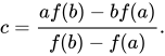
False position is similar to the secant method, except that, instead of retaining the last two points, it makes sure to keep one point on either side of the root. The false position method can be faster than the bisection method and will never diverge like the secant method. However, it may fail to converge in some naive implementations due to roundoff errors that may lead to a wrong sign for f(c). Typically, this may occur if the derivative of f is large in the neighborhood of the root.
Interpolation
Many root-finding processes work by interpolation. This consists in using the last computed approximate values of the root for approximating the function by a polynomial of low degree, which takes the same values at these approximate roots. Then the root of the polynomial is computed and used as a new approximate value of the root of the function, and the process is iterated.
Interpolating two values yields a line: a polynomial of degree one. This is the basis of the secant method. Regula falsi is also an interpolation method that interpolates two points at a time but it differs from the secant method by using two points that are not necessarily the last two computed points. Three values define a parabolic curve: a quadratic function. This is the basis of Muller's method.
Iterative methods
Although all root-finding algorithms proceed by iteration, an iterative root-finding method generally uses a specific type of iteration, consisting of defining an auxiliary function, which is applied to the last computed approximations of a root for getting a new approximation. The iteration stops when a fixed point of the auxiliary function is reached to the desired precision, i.e., when a new computed value is sufficiently close to the preceding ones.
Newton's method (and similar derivative-based methods)
Newton's method assumes the function f to have a continuous derivative. Newton's method may not converge if started too far away from a root. However, when it does converge, it is faster than the bisection method; its order of convergence is usually quadratic whereas the bisection method's is linear. Newton's method is also important because it readily generalizes to higher-dimensional problems. Householder's methods are a class of Newton-like methods with higher orders of convergence. The first one after Newton's method is Halley's method with cubic order of convergence.
Secant method
Replacing the derivative in Newton's method with a finite difference, we get the secant method. This method does not require the computation (nor the existence) of a derivative, but the price is slower convergence (the order of convergence is the golden ratio, approximately 1.62[2]). A generalization of the secant method in higher dimensions is Broyden's method.
Steffensen's method
If we use a polynomial fit to remove the quadratic part of the finite difference used in the secant method, so that it better approximates the derivative, we obtain Steffensen's method, which has quadratic convergence, and whose behavior (both good and bad) is essentially the same as Newton's method but does not require a derivative.
Fixed point iteration method
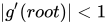
We can use the fixed-point iteration to find the root of a function. Given a function which we have set to zero to find the root (), we rewrite the equation in terms of so that becomes (note, there are often many functions for each function). Next, we relabel each side of the equation as so that we can perform the iteration. Next, we pick a value for and perform the iteration until it converges towards a root of the function. If the iteration converges, it will converge to a root. The iteration will only converge if .


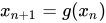

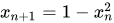
As an example of converting to , if given the function , we will rewrite it as one of the following equations.

- ,
- ,
- ,
- , or
- .




Inverse interpolation
The appearance of complex values in interpolation methods can be avoided by interpolating the inverse of f, resulting in the inverse quadratic interpolation method. Again, convergence is asymptotically faster than the secant method, but inverse quadratic interpolation often behaves poorly when the iterates are not close to the root.
Combinations of methods
Brent's method
Brent's method is a combination of the bisection method, the secant method and inverse quadratic interpolation. At every iteration, Brent's method decides which method out of these three is likely to do best, and proceeds by doing a step according to that method. This gives a robust and fast method, which therefore enjoys considerable popularity.
Ridders' method
Ridders' method is a hybrid method that uses the value of function at the midpoint of the interval to perform an exponential interpolation to the root. This gives a fast convergence with a guaranteed convergence of at most twice the number of iterations as the bisection method.
Roots of polynomials
Finding the roots of polynomials is a long-standing problem that has been extensively studied throughout the history and substantially influenced the development of mathematics. It involves determining either a numerical approximation or a closed-form expression of the roots of a univariate polynomial, i.e., determining approximate or closed form solutions of in the equation

where are either real or complex numbers.

Efforts to understand and solve polynomial equations led to the development of important mathematical concepts, including irrational and complex numbers, as well as foundational structures in modern algebra such as fields, rings, and groups.
Despite being historically important, finding the roots of higher degree polynomials no longer play a central role in mathematics and computational mathematics, with one major exception in computer algebra.[3]
Finding roots in higher dimensions
The bisection method has been generalized to higher dimensions; these methods are called generalized bisection methods.[4][5] At each iteration, the domain is partitioned into two parts, and the algorithm decides - based on a small number of function evaluations - which of these two parts must contain a root. In one dimension, the criterion for decision is that the function has opposite signs. The main challenge in extending the method to multiple dimensions is to find a criterion that can be computed easily and guarantees the existence of a root.
The Poincaré–Miranda theorem gives a criterion for the existence of a root in a rectangle, but it is hard to verify because it requires evaluating the function on the entire boundary of the rectangle.
Another criterion is given by a theorem of Kronecker.[6] It says that, if the topological degree of a function f on a rectangle is non-zero, then the rectangle must contain at least one root of f. This criterion is the basis for several root-finding methods, such as those of Stenger[7] and Kearfott.[8] However, computing the topological degree can be time-consuming.
A third criterion is based on a characteristic polyhedron. This criterion is used by a method called Characteristic Bisection.[4]:19-- It does not require computing the topological degree; it only requires computing the signs of function values. The number of required evaluations is at least , where D is the length of the longest edge of the characteristic polyhedron.[9]:11,Lemma.4.7 Note that Vrahatis and Iordanidis [9] prove a lower bound on the number of evaluations, and not an upper bound.

A fourth method uses an intermediate value theorem on simplices.[10] Again, no upper bound on the number of queries is given.
See also
Broyden's method – Quasi-Newton root-finding method for the multivariable case
- Cryptographically secure pseudorandom number generator – Type of functions designed for being unsolvable by root-finding algorithms
- GNU Scientific Library
- Graeffe's method – Algorithm for finding polynomial roots
- Método de Lill : método gráfico para hallar las raíces reales de un polinomio.
- MPSolve : software para aproximar las raíces de un polinomio con una precisión arbitrariamente alta.
- Multiplicidad (matemáticas) : Número de veces que un objeto debe contarse para que una fórmula general sea verdadera.
- algoritmo de la raíz n -ésima
- Sistema de ecuaciones polinómicas – Raíces de polinomios multivariables múltiples
- Teorema de Kantorovich – Sobre la convergencia del método de Newton
Referencias
- ↑ Press, WH; Teukolsky, SA; Vetterling, WT; Flannery, BP (2007). «Capítulo 9. Búsqueda de raíces y sistemas de ecuaciones no lineales» . Numerical Recipes: The Art of Scientific Computing (3.ª ed.). Nueva York: Cambridge University Press. ISBN 978-0-521-88068-8.
- ↑ Chanson, Jeffrey R. (3 de octubre de 2024). "Orden de convergencia" . LibreTexts Mathematics . Recuperado el 3 de octubre de 2024 .
- ↑ Pan, Victor Y. (enero de 1997). "Resolución de una ecuación polinómica: algunos antecedentes y avances recientes" . SIAM Review . 39 (2): 187– 220. doi : 10.1137/S0036144595288554 . ISSN 0036-1445 .
- 1 2 Mourrain, B.; Vrahatis, MN; Yakoubsohn, JC (2002-06-01). "Sobre la complejidad de aislar raíces reales y calcular con certeza el grado topológico" . Journal of Complexity . 18 (2): 612– 640. doi : 10.1006/jcom.2001.0636 . ISSN 0885-064X .
- ↑ Vrahatis, Michael N. (2020). "Generalizaciones del teorema del valor intermedio para aproximar puntos fijos y ceros de funciones continuas" . En Sergeyev, Yaroslav D.; Kvasov, Dmitri E. (eds.). Computación numérica: teoría y algoritmos . Lecture Notes in Computer Science. Vol. 11974. Cham: Springer International Publishing. pp. 223–238 . doi : 10.1007/978-3-030-40616-5_17 . ISBN 978-3-030-40616-5. S2CID 211160947 .
- ↑ Ortega, James M.; Rheinboldt, Werner C. (2000). Solución iterativa de ecuaciones no lineales en varias variables . Society for Industrial and Applied Mathematics. ISBN 978-0-89871-461-6.
- ↑ Stenger, Frank (1975-03-01). "Cálculo del grado topológico de una aplicación en Rn". Numerische Mathematik . 25 (1): 23– 38. doi : 10.1007/BF01419526 . ISSN 0945-3245 . S2CID 122196773 .
- ↑ Kearfott, Baker (1979-06-01). "Un método eficiente de cálculo de grados para un método generalizado de bisección". Numerische Mathematik . 32 (2): 109– 127. doi : 10.1007/BF01404868 . ISSN 0029-599X . S2CID 122058552 .
- 1 2 Vrahatis, MN; Iordanidis, KI (1986-03-01). "Un método generalizado rápido de bisección para resolver sistemas de ecuaciones no lineales". Numerische Mathematik . 49 (2): 123– 138. doi : 10.1007/BF01389620 . ISSN 0945-3245 . S2CID 121771945 .
- ↑ Vrahatis, Michael N. (15 de abril de 2020). "Teorema del valor intermedio para símplices para la aproximación simplicial de puntos fijos y ceros" . Topology and Its Applications . 275 107036. doi : 10.1016/j.topol.2019.107036 . ISSN 0166-8641 . S2CID 213249321 .
Lecturas adicionales
- Victor Yakovlevich Pan: "Resolución de una ecuación polinómica: algunos antecedentes y avances recientes", SIAM Review, vol. 39, n.º 2, págs. 187-220 (junio de 1997).
- John Michael McNamee: Métodos numéricos para raíces de polinomios - Parte I , Elsevier, ISBN 978-0-444-52729-5 (2007).
- John Michael McNamee y Victor Yakovlevich Pan: Métodos numéricos para raíces de polinomios - Parte II , Elsevier, ISBN 978-0-444-52730-1 (2013).
- Algoritmos para la búsqueda de raíces