 Hispanopedia Wiki
In mathematical analysis, p-variation is a collection of seminorms on functions from an ordered set to a metric space, indexed by a real number . p-variation is a measure of the regularity or smoothness of a function. Specifically, if , where is a metric space and I a totally ordered set, its p-variation is




where D ranges over all finite partitions of the interval I.
The p variation of a function decreases with p. If f has finite p-variation and g is an α-Hölder continuous function, then has finite -variation.


The case when p is one is called total variation, and functions with a finite 1-variation are called bounded variation functions.
Link with Hölder norm
One can interpret the p-variation as a parameter-independent version of the Hölder norm, which also extends to discontinuous functions.
If f is α–Hölder continuous (i.e. its α–Hölder norm is finite) then its -variation is finite. Specifically, on an interval [a,b], .


Conversely, if f is continuous and has finite p-variation, there exists a reparameterisation, , such that is Hölder continuous.[1]


If p is less than q then the space of functions of finite p-variation on a compact set is continuously embedded with norm 1 into those of finite q-variation. I.e. . However unlike the analogous situation with Hölder spaces the embedding is not compact. For example, consider the real functions on [0,1] given by . They are uniformly bounded in 1-variation and converge pointwise to a discontinuous function f but this not only is not a convergence in p-variation for any p but also is not uniform convergence.


Application to Riemann–Stieltjes integration
If f and g are functions from [a, b] to with no common discontinuities and with f having finite p-variation and g having finite q-variation, with then the Riemann–Stieltjes Integral


![{\displaystyle \int _{a}^{b}f(x)\,dg(x):=\lim _{|D|\to 0}\sum _{t_{k}\in D}f(t_{k})[g(t_{k+1})-g({t_{k}})]}](https://wikimedia.org/api/rest_v1/media/math/render/svg/046ee86b11a58ef6c7fec463cd9defd57ba7fdde)
is well-defined. This integral is known as the Young integral because it comes from Young (1936).[2] The value of this definite integral is bounded by the Young-Loève estimate as follows
![{\displaystyle \left|\int _{a}^{b}f(x)\,dg(x)-f(\xi )[g(b)-g(a)]\right|\leq C\,\|f\|_{p{\text{-var}}}\|\,g\|_{q{\text{-var}}}}](https://wikimedia.org/api/rest_v1/media/math/render/svg/db6731ad2770e656cb57833595b25e3c9a2d2b7b)
where C is a constant which only depends on p and q and ξ is any number between a and b.[3] If f and g are continuous, the indefinite integral is a continuous function with finite q-variation: If a ≤ s ≤ t ≤ b then , its q-variation on [s,t], is bounded by where C is a constant which only depends on p and q.[4]
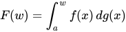
![{\displaystyle \|F\|_{q{\text{-var}};[s,t]}}](https://wikimedia.org/api/rest_v1/media/math/render/svg/29de4a2c81ecbc20d8b5d48e4509323e15d8a9ac)
![{\displaystyle C\|g\|_{q{\text{-var}};[s,t]}(\|f\|_{p{\text{-var}};[s,t]}+\|f\|_{\infty ;[s,t]})\leq 2C\|g\|_{q{\text{-var}};[s,t]}(\|f\|_{p{\text{-var}};[a,b]}+f(a))}](https://wikimedia.org/api/rest_v1/media/math/render/svg/5bd454c6633a99ebb81edfd014b9169d3ffe9a14)
Differential equations driven by signals of finite p-variation, p < 2
A function from to e × d real matrices is called an -valued one-form on .


If f is a Lipschitz continuous -valued one-form on , and X is a continuous function from the interval [a, b] to with finite p-variation with p less than 2, then the integral of f on X, , can be calculated because each component of f(X(t)) will be a path of finite p-variation and the integral is a sum of finitely many Young integrals. It provides the solution to the equation driven by the path X.
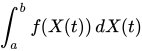

More significantly, if f is a Lipschitz continuous -valued one-form on , and X is a continuous function from the interval [a, b] to with finite p-variation with p less than 2, then Young integration is enough to establish the solution of the equation driven by the path X.[5]

Differential equations driven by signals of finite p-variation, p ≥ 2
The theory of rough paths generalises the Young integral and Young differential equations and makes heavy use of the concept of p-variation.
For Brownian motion
p-variation should be contrasted with the quadratic variation which is used in stochastic analysis, which takes one stochastic process to another. In particular the definition of quadratic variation looks a bit like the definition of p-variation, when p has the value 2. Quadratic variation is defined as a limit as the partition gets finer, whereas p-variation is a supremum over all partitions. Thus the quadratic variation of a process could be smaller than its 2-variation. If Wt is a standard Brownian motion on [0, T], then with probability one its p-variation is infinite for and finite otherwise. The quadratic variation of W is .

![{\displaystyle [W]_{T}=T}](https://wikimedia.org/api/rest_v1/media/math/render/svg/8af2af4c43ea2fe7421d314221d4549e22d9007f)
Computation of p-variation for discrete time series
For a discrete time series of observations X0,...,XN it is straightforward to compute its p-variation with complexity of O(N2). Here is an example C++ code using dynamic programming:
double p_var(const std::vector<double>& X, double p) {
	if (X.size() == 0)
		return 0.0;
	std::vector<double> cum_p_var(X.size(), 0.0);   // cumulative p-variation
	for (size_t n = 1; n < X.size(); n++) {
		for (size_t k = 0; k < n; k++) {
			cum_p_var[n] = std::max(cum_p_var[n], cum_p_var[k] + std::pow(std::abs(X[n] - X[k]), p));
		}
	}
	return std::pow(cum_p_var.back(), 1./p);
}
There exist much more efficient, but also more complicated, algorithms for -valued processes[6] [7] and for processes in arbitrary metric spaces.[7]
References
- ^ Ullrich, David C. (27 Feb 2018). "real analysis - Link between p-variation and Hölder norm". Mathematics Stack Exchange. Retrieved 2021-07-02.
- ^ "Lecture 7. Young's integral". 25 December 2012.
- ^ Friz, Peter K.; Victoir, Nicolas (2010). Multidimensional Stochastic Processes as Rough Paths: Theory and Applications (Cambridge Studies in Advanced Mathematics ed.). Cambridge University Press.
- ^ Lyons, Terry; Caruana, Michael; Levy, Thierry (2007). Differential equations driven by rough paths, vol. 1908 of Lecture Notes in Mathematics. Springer.
- ^ "Lecture 8. Young's differential equations". 26 December 2012.
- ^ Butkus, V.; Norvaiša, R. (2018). "Computation of p-variation". Lithuanian Mathematical Journal. 58 (4): 360–378. doi:10.1007/s10986-018-9414-3. S2CID 126246235.
- ^ a b "P-var". GitHub. 8 May 2020.
- Young, L.C. (1936), "An inequality of the Hölder type, connected with Stieltjes integration", Acta Mathematica, 67 (1): 251–282, doi:10.1007/bf02401743.
External links
- Continuous Paths with bounded p-variation Fabrice Baudoin
- On the Young integral, truncated variation and rough paths Rafał M. Łochowski