Genus of a multiplicative sequence

In mathematics, a genus of a multiplicative sequence is a ring homomorphism from the ring of smooth compact manifolds up to the equivalence of bounding a smooth manifold with boundary (i.e., up to suitable cobordism) to another ring, usually the rational numbers, having the property that they are constructed from a sequence of polynomials in characteristic classes that arise as coefficients in formal power series with good multiplicative properties.

A genus${\displaystyle \varphi }$ assigns a number ${\displaystyle \Phi (X)}$ to each manifold X such that

1. ${\displaystyle \Phi (X\sqcup Y)=\Phi (X)+\Phi (Y)}$ (where ${\displaystyle \sqcup }$ is the disjoint union);
2. ${\displaystyle \Phi (X\times Y)=\Phi (X)\Phi (Y)}$;
3. ${\displaystyle \Phi (X)=0}$ if X is the boundary of a manifold with boundary.

The manifolds and manifolds with boundary may be required to have additional structure; for example, they might be oriented, spin, stably complex, and so on (see list of cobordism theories for many more examples). The value ${\displaystyle \Phi (X)}$ is in some ring, often the ring of rational numbers, though it can be other rings such as ${\displaystyle \mathbb {Z} /2\mathbb {Z} }$ or the ring of modular forms.

The conditions on ${\displaystyle \Phi }$ can be rephrased as saying that ${\displaystyle \Phi }$ is a ring homomorphism from the cobordism ring of manifolds (with additional structure) to another ring.

Example: If ${\displaystyle \Phi (X)}$ is the signature of the oriented manifold X, then ${\displaystyle \Phi }$ is a genus from oriented manifolds to the ring of integers.

A sequence of polynomials ${\displaystyle K_{1},K_{2},\ldots }$ in variables ${\displaystyle p_{1},p_{2},\ldots }$ is called multiplicative if

${\displaystyle 1+p_{1}z+p_{2}z^{2}+\cdots =(1+q_{1}z+q_{2}z^{2}+\cdots )(1+r_{1}z+r_{2}z^{2}+\cdots )}$

implies that

${\displaystyle \sum _{j}K_{j}(p_{1},p_{2},\ldots )z^{j}=\sum _{j}K_{j}(q_{1},q_{2},\ldots )z^{j}\sum _{k}K_{k}(r_{1},r_{2},\ldots )z^{k}}$

If ${\displaystyle Q(z)}$ is a formal power series in z with constant term 1, we can define a multiplicative sequence

${\displaystyle K=1+K_{1}+K_{2}+\cdots }$

by

${\displaystyle K(p_{1},p_{2},p_{3},\ldots )=Q(z_{1})Q(z_{2})Q(z_{3})\cdots }$,

where ${\displaystyle p_{k}}$ is the kth elementary symmetric function of the indeterminates ${\displaystyle z_{i}}$. (The variables ${\displaystyle p_{k}}$ will often in practice be Pontryagin classes.)

The genus ${\displaystyle \Phi }$ of compact, connected, smooth, oriented manifolds corresponding to Q is given by

${\displaystyle \Phi (X)=K(p_{1},p_{2},p_{3},\ldots )}$

where the ${\displaystyle p_{k}}$ are the Pontryagin classes of X. The power series Q is called the characteristic power series of the genus ${\displaystyle \Phi }$. A theorem of René Thom, which states that the rationals tensored with the cobordism ring is a polynomial algebra in generators of degree 4k for positive integers k, implies that this gives a bijection between formal power series Q with rational coefficients and leading coefficient 1, and genera from oriented manifolds to the rational numbers.

The L genus is the genus of the formal power series

${\displaystyle {{\sqrt {z}} \over \tanh({\sqrt {z}})}=\sum _{k\geq 0}{\frac {2^{2k}B_{2k}z^{k}}{(2k)!}}=1+{z \over 3}-{z^{2} \over 45}+\cdots }$

where the numbers ${\displaystyle B_{2k}}$ are the Bernoulli numbers. The first few values are:

${\displaystyle {\begin{aligned}L_{0}&=1\\L_{1}&={\tfrac {1}{3}}p_{1}\\L_{2}&={\tfrac {1}{45}}\left(7p_{2}-p_{1}^{2}\right)\\L_{3}&={\tfrac {1}{945}}\left(62p_{3}-13p_{1}p_{2}+2p_{1}^{3}\right)\\L_{4}&={\tfrac {1}{14175}}\left(381p_{4}-71p_{1}p_{3}-19p_{2}^{2}+22p_{1}^{2}p_{2}-3p_{1}^{4}\right)\end{aligned}}}$

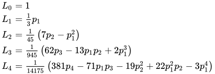
(for further L-polynomials see ^[1] or OEIS: A237111). Now let M be a closed smooth oriented manifold of dimension 4n with Pontrjagin classes${\displaystyle p_{i}=p_{i}(M)}$. Friedrich Hirzebruch showed that the L genus of M in dimension 4n evaluated on the fundamental class of ${\displaystyle M}$, denoted ${\displaystyle [M]}$, is equal to ${\displaystyle \sigma (M)}$, the signature of M (i.e., the signature of the intersection form on the 2nth cohomology group of M):

${\displaystyle \sigma (M)=\langle L_{n}(p_{1}(M),\ldots ,p_{n}(M)),[M]\rangle }$.

This is now known as the Hirzebruch signature theorem (or sometimes the Hirzebruch index theorem).

The fact that ${\displaystyle L_{2}}$ is always integral for a smooth manifold was used by John Milnor to give an example of an 8-dimensional piecewise linear (PL) manifold with no smooth structure. Pontryagin numbers can also be defined for PL manifolds, and Milnor showed that his PL manifold had a non-integral value of ${\displaystyle p_{2}}$, and so was not smoothable.

The Todd genus is the genus of the formal power series

${\displaystyle {\frac {z}{1-\exp(-z)}}=\sum _{i=0}^{\infty }{\frac {B_{i}}{i!}}z^{i}}$

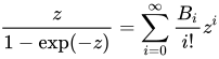
with ${\displaystyle B_{i}}$ as before, Bernoulli numbers. The first few values are

${\displaystyle {\begin{aligned}Td_{0}&=1\\Td_{1}&={\frac {1}{2}}c_{1}\\Td_{2}&={\frac {1}{12}}\left(c_{2}+c_{1}^{2}\right)\\Td_{3}&={\frac {1}{24}}c_{1}c_{2}\\Td_{4}&={\frac {1}{720}}\left(-c_{1}^{4}+4c_{2}c_{1}^{2}+3c_{2}^{2}+c_{3}c_{1}-c_{4}\right)\end{aligned}}}$

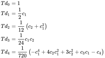
The Todd genus has the particular property that it assigns the value 1 to all complex projective spaces (i.e. ${\displaystyle \mathrm {Td} _{n}(\mathbb {CP} ^{n})=1}$), y esto basta para demostrar que el género de Todd coincide con el género aritmético para variedades algebraicas , ya que el género aritmético también es 1 para espacios proyectivos complejos. Esta observación es consecuencia del teorema de Hirzebruch-Riemann-Roch y, de hecho, es uno de los desarrollos clave que condujeron a la formulación de dicho teorema.

El género es el género asociado a la serie de potencias característica.

${\displaystyle Q(z)={\frac {{\frac {1}{2}}{\sqrt {z}}}{\sinh \left({\frac {1}{2}}{\sqrt {z}}\right)}}=1-{\frac {z}{24}}+{\frac {7z^{2}}{5760}}-\cdots }$

(También existe un género A que se usa con menos frecuencia, asociado a la serie característica.${\displaystyle Q(16z)}$.) Los primeros valores son

${\displaystyle {\begin{aligned}{\hat {A}}_{0}&=1\\{\hat {A}}_{1}&=-{\tfrac {1}{24}}p_{1}\\{\hat {A}}_{2}&={\tfrac {1}{5760}}\left(-4p_{2}+7p_{1}^{2}\right)\\{\hat {A}}_{3}&={\tfrac {1}{967680}}\left(-16p_{3}+44p_{2}p_{1}-31p_{1}^{3}\right)\\{\hat {A}}_{4}&={\tfrac {1}{464486400}}\left(-192p_{4}+512p_{3}p_{1}+208p_{2}^{2}-904p_{2}p_{1}^{2}+381p_{1}^{4}\right)\end{aligned}}}$

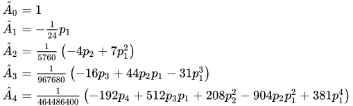
El género de una variedad de espín es un entero, y un entero par si la dimensión es 4 mod 8 (lo que en dimensión 4 implica el teorema de Rochlin ); para variedades generales, el género no siempre es un entero. Esto fue demostrado por Hirzebruch y Armand Borel ; este resultado fue motivado y posteriormente explicado por el teorema del índice de Atiyah-Singer , que mostró que el género de una variedad de espín es igual al índice de su operador de Dirac .

Al combinar este resultado del índice con una fórmula de Weitzenbock para el laplaciano de Dirac, André Lichnerowicz dedujo que si una variedad de espín compacta admite una métrica con curvatura escalar positiva , su género  debe anularse. Esto solo proporciona una obstrucción a la curvatura escalar positiva cuando la dimensión es un múltiplo de 4, pero Nigel Hitchin descubrió más tarde un análogo.${\displaystyle \mathbb {Z} _{2}}$obstrucción con valor en dimensiones 1 o 2 mod 8. Estos resultados son esencialmente precisos. De hecho, Mikhail Gromov , H. Blaine Lawson y Stephan Stolz demostraron posteriormente que el género  y el de Hitchin${\displaystyle \mathbb {Z} _{2}}$Los análogos con valores son las únicas obstrucciones a la existencia de métricas de curvatura escalar positiva en variedades de espín simplemente conexas de dimensión mayor o igual a 5.

Un género se denomina género elíptico si la serie de potencias${\displaystyle Q(z)=z/f(z)}$satisface la condición

${\displaystyle {f'}^{2}=1-2\delta f^{2}+\epsilon f^{4}}$

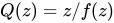
para constantes${\displaystyle \delta }$y${\displaystyle \epsilon }$(Como es habitual, Q es la serie de potencias característica del género).

Una expresión explícita para f ( z ) es

${\displaystyle f(z)={\frac {1}{a}}\operatorname {sn} \left(az,{\frac {\sqrt {\epsilon }}{a^{2}}}\right)}$

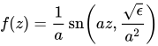
dónde

${\displaystyle a={\sqrt {\delta +{\sqrt {\delta ^{2}-\epsilon }}}}}$

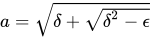
y sn es la función elíptica de Jacobi .

Ejemplos:

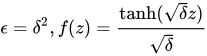
• ${\displaystyle \delta =\epsilon =1,f(z)=\tanh(z)}$Este es el género L.
• ${\displaystyle \delta =-{\frac {1}{8}},\epsilon =0,f(z)=2\sinh \left({\frac {1}{2}}z\right)}$Este es el género.
• ${\displaystyle \epsilon =\delta ^{2},f(z)={\frac {\tanh({\sqrt {\delta }}z)}{\sqrt {\delta }}}}$. Esta es una generalización del género L.

Los primeros valores de dichos géneros son:

${\displaystyle {\frac {1}{3}}\delta p_{1}}$

${\displaystyle {\frac {1}{90}}\left[\left(-4\delta ^{2}+18\epsilon \right)p_{2}+\left(7\delta ^{2}-9\epsilon \right)p_{1}^{2}\right]}$

${\displaystyle {\frac {1}{1890}}\left[\left(16\delta ^{3}+108\delta \epsilon \right)p_{3}+\left(-44\delta ^{3}+18\delta \epsilon \right)p_{2}p_{1}+\left(31\delta ^{3}-27\delta \epsilon \right)p_{1}^{3}\right]}$

Ejemplo (género elíptico para plano proyectivo cuaterniónico )  :

${\displaystyle {\begin{aligned}\Phi _{ell}(HP^{2})&=\int _{HP^{2}}{\tfrac {1}{90}}{\big [}(-4\delta ^{2}+18\epsilon )p_{2}+(7\delta ^{2}-9\epsilon )p_{1}^{2}{\big ]}\\&=\int _{HP^{2}}{\tfrac {1}{90}}{\big [}(-4\delta ^{2}+18\epsilon )(7u^{2})+(7\delta ^{2}-9\epsilon )(2u)^{2}{\big ]}\\&=\int _{HP^{2}}[u^{2}\epsilon ]\\&=\epsilon \int _{HP^{2}}[u^{2}]\\&=\epsilon *1=\epsilon \end{aligned}}}$

Ejemplo (género elíptico para el plano proyectivo octoniónico, o plano de Cayley ):

${\displaystyle {\begin{aligned}\Phi _{ell}(OP^{2})&=\int _{OP^{2}}{\tfrac {1}{113400}}\left[(-192\delta ^{4}+1728\delta ^{2}\epsilon +1512\epsilon ^{2})p_{4}+(208\delta ^{4}-1872\delta ^{2}\epsilon +1512\epsilon ^{2})p_{2}^{2}\right]\\&=\int _{OP^{2}}{\tfrac {1}{113400}}{\big [}(-192\delta ^{4}+1728\delta ^{2}\epsilon +1512\epsilon ^{2})(39u^{2})+(208\delta ^{4}-1872\delta ^{2}\epsilon +1512\epsilon ^{2})(6u)^{2}{\big ]}\\&=\int _{OP^{2}}{\big [}\epsilon ^{2}u^{2}{\big ]}\\&=\epsilon ^{2}\int _{OP^{2}}{\big [}u^{2}{\big ]}\\&=\epsilon ^{2}*1=\epsilon ^{2}\\&=\Phi _{ell}(HP^{2})^{2}\end{aligned}}}$

El género de Witten es el género asociado a la serie de potencias característica.

${\displaystyle Q(z)={\frac {z}{\sigma _{L}(z)}}=\exp \left(\sum _{k\geq 2}{2G_{2k}(\tau )z^{2k} \over (2k)!}\right)}$

donde σ _L es la función sigma de Weierstrass para la red L , y G es un múltiplo de una serie de Eisenstein .

El género de Witten de una variedad de espín suave orientada y compacta de 4k dimensiones con primera clase de Pontryagin nula es una forma modular de peso 2k , con coeficientes de Fourier enteros.

• Teorema del índice de Atiyah-Singer
• Lista de teorías de cohomología

• Friedrich Hirzebruch Métodos topológicos en geometría algebraica ISBN 3-540-58663-6Texto de la versión original en alemán: http://hirzebruch.mpim-bonn.mpg.de/120/6/NeueTopologischeMethoden_2.Aufl.pdf
• Friedrich Hirzebruch, Thomas Berger, Rainer Jung Variedades y formas modulares ISBN 3-528-06414-5
• Milnor, John W.; Stasheff , James D. (1974). Clases características . Annals of Mathematics Studies. Vol.  76. Princeton University Press; University of Tokyo Press. ISBN 978-0-691-08122-9. MR 0440554 . 
• AF Kharshiladze (2001) [1994], "Clase Pontryagin" , Enciclopedia de Matemáticas , EMS Press
• "Géneros elípticos" , Enciclopedia de Matemáticas , EMS Press , 2001 [1994]