Dual Hahn polynomials

In mathematics, the dual Hahn polynomials are a family of orthogonal polynomials in the Askey scheme of hypergeometric orthogonal polynomials. They are defined on a non-uniform lattice ${\displaystyle x(s)=s(s+1)}$ and are defined as

${\displaystyle w_{n}^{(c)}(s,a,b)={\frac {(a-b+1)_{n}(a+c+1)_{n}}{n!}}{}_{3}F_{2}(-n,a-s,a+s+1;a-b+a,a+c+1;1)}$

for ${\displaystyle n=0,1,...,N-1}$ and the parameters ${\displaystyle a,b,c}$ are restricted to ${\displaystyle -{\frac {1}{2}}<a<b,|c|<1+a,b=a+N}$.

Note that ${\displaystyle (u)_{k}}$ is the rising factorial, otherwise known as the Pochhammer symbol, and ${\displaystyle {}_{3}F_{2}(\cdot )}$ is the generalized hypergeometric functions

RoelofKoekoek,Peter A. Lesky,andRené F. Swarttouw (2010,14) give a detailed list of their properties.

The dual Hahn polynomials have the orthogonality condition

${\displaystyle \sum _{s=a}^{b-1}w_{n}^{(c)}(s,a,b)w_{m}^{(c)}(s,a,b)\rho (s)[\Delta x(s-{\frac {1}{2}})]=\delta _{nm}d_{n}^{2}}$

for ${\displaystyle n,m=0,1,...,N-1}$. Where ${\displaystyle \Delta x(s)=x(s+1)-x(s)}$,

${\displaystyle \rho (s)={\frac {\Gamma (a+s+1)\Gamma (c+s+1)}{\Gamma (s-a+1)\Gamma (b-s)\Gamma (b+s+1)\Gamma (s-c+1)}}}$

and

${\displaystyle d_{n}^{2}={\frac {\Gamma (a+c+n+a)}{n!(b-a-n-1)!\Gamma (b-c-n)}}.}$

As the value of ${\displaystyle n}$ increases, the values that the discrete polynomials obtain also increases. As a result, to obtain numerical stability in calculating the polynomials you would use the renormalized dual Hahn polynomial as defined as

${\displaystyle {\hat {w}}_{n}^{(c)}(s,a,b)=w_{n}^{(c)}(s,a,b){\sqrt {{\frac {\rho (s)}{d_{n}^{2}}}[\Delta x(s-{\frac {1}{2}})]}}}$

for ${\displaystyle n=0,1,...,N-1}$.

Then the orthogonality condition becomes

${\displaystyle \sum _{s=a}^{b-1}{\hat {w}}_{n}^{(c)}(s,a,b){\hat {w}}_{m}^{(c)}(s,a,b)=\delta _{m,n}}$

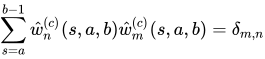
for ${\displaystyle n,m=0,1,...,N-1}$

The Hahn polynomials, ${\displaystyle h_{n}(x,N;\alpha ,\beta )}$, is defined on the uniform lattice ${\displaystyle x(s)=s}$, and the parameters ${\displaystyle a,b,c}$ are defined as ${\displaystyle a=(\alpha +\beta )/2,b=a+N,c=(\beta -\alpha )/2}$. Then setting ${\displaystyle \alpha =\beta =0}$ the Hahn polynomials become the Chebyshev polynomials. Note that the dual Hahn polynomials have a q-analog with an extra parameter q known as the dual q-Hahn polynomials.

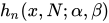
Racah polynomials are a generalization of dual Hahn polynomials.

• Zhu, Hongqing (2007), "Image analysis by discrete orthogonal dual Hahn moments"(PDF), Pattern Recognition Letters, 28 (13): 1688–1704, doi:10.1016/j.patrec.2007.04.013
• Hahn, Wolfgang (1949), "Über Orthogonalpolynome, die q-Differenzengleichungen genügen", Mathematische Nachrichten, 2 (1–2): 4–34, doi:10.1002/mana.19490020103, ISSN 0025-584X, MR 0030647
• Koekoek, Roelof; Lesky, Peter A.; Swarttouw, René F. (2010), Hypergeometric orthogonal polynomials and their q-analogues, Springer Monographs in Mathematics, Berlin, New York: Springer-Verlag, doi:10.1007/978-3-642-05014-5, ISBN 978-3-642-05013-8, MR 2656096
• Koornwinder, Tom H.; Wong, Roderick SC; Koekoek, Roelof; Swarttouw, René F. (2010), "Clase Hahn: Definiciones" , en Olver, Frank WJ ; Lozier, Daniel M.; Boisvert, Ronald F.; Clark, Charles W. (eds.), Manual de funciones matemáticas del NIST , Cambridge University Press, ISBN 978-0-521-19225-5, MR 2723248 .