Articulo de referencia

Función modular Weber

En matemáticas , las funciones modulares de Weber son una familia de tres funciones f , f 1 y f 2 , [nota 1] estudiadas por Heinrich Martin Weber . Definición Sea donde τ es un ...

En matemáticas , las funciones modulares de Weber son una familia de tres funciones f , f 1 y f 2 , [nota 1] estudiadas por Heinrich Martin Weber .

Definición

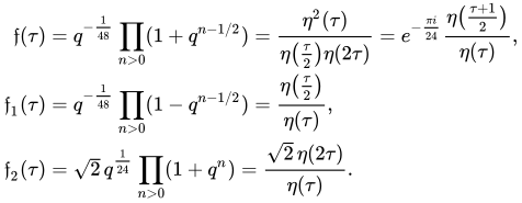
Sea donde τ es un elemento del semiplano superior . Entonces las funciones de Weber son q = mi 2 π i τ {\displaystyle q=e^{2\pi i\tau}}

F ( τ ) = q 1 48 norte > 0 ( 1 + q norte 1 / 2 ) = η 2 ( τ ) η ( τ 2 ) η ( 2 τ ) = mi π i 24 η ( τ + 1 2 ) η ( τ ) , F 1 ( τ ) = q 1 48 norte > 0 ( 1 q norte 1 / 2 ) = η ( τ 2 ) η ( τ ) , F 2 ( τ ) = 2 q 1 24 norte > 0 ( 1 + q norte ) = 2 η ( 2 τ ) η ( τ ) . {\displaystyle {\begin{aligned}{\mathfrak {f}}(\tau )&=q^{-{\frac {1}{48}}}\prod _{n>0}(1+q^{n-1/2})={\frac {\eta ^{2}(\tau )}{\eta {\big (}{\tfrac {\tau }{2}}{\big )}\eta (2\tau )}}=e^{-{\frac {\pi i}{24}}}{\frac {\eta {\big (}{\frac {\tau +1}{2}}{\big )}}{\eta (\tau )}},\\{\mathfrak {f}}_{1}(\tau )&=q^{-{\frac {1}{48}}}\prod _{n>0}(1-q^{n-1/2})={\frac {\eta {\big (}{\tfrac {\tau }{2}}{\big )}}{\eta (\tau )}},\\{\mathfrak {f}}_{2}(\tau )&={\sqrt {2}}\,q^{\frac {1}{24}}\prod _{n>0}(1+q^{n})={\frac {{\sqrt {2}}\,\eta (2\tau )}{\eta (\tau )}}.\end{aligned}}}

Estas son también las definiciones del artículo de Duke "Fracciones continuas y funciones modulares" . [nota 2] La función es la función eta de Dedekind y debe interpretarse como . Las descripciones como cocientes implican inmediatamente η ( τ ) {\displaystyle \eta (\tau )} ( e 2 π i τ ) α {\displaystyle (e^{2\pi i\tau })^{\alpha }} e 2 π i τ α {\displaystyle e^{2\pi i\tau \alpha }} η {\displaystyle \eta }

f ( τ ) f 1 ( τ ) f 2 ( τ ) = 2 . {\displaystyle {\mathfrak {f}}(\tau ){\mathfrak {f}}_{1}(\tau ){\mathfrak {f}}_{2}(\tau )={\sqrt {2}}.}

La transformación τ  → –1/ τ fija f e intercambia f 1 y f 2 . Por lo tanto, el espacio vectorial complejo tridimensional con base f , f 1 y f 2 se ve afectado por el grupo SL 2 ( Z ).

Producto infinito alternativo

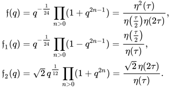
Alternativamente, sea el nombre , q = e π i τ {\displaystyle q=e^{\pi i\tau }}

f ( q ) = q 1 24 n > 0 ( 1 + q 2 n 1 ) = η 2 ( τ ) η ( τ 2 ) η ( 2 τ ) , f 1 ( q ) = q 1 24 n > 0 ( 1 q 2 n 1 ) = η ( τ 2 ) η ( τ ) , f 2 ( q ) = 2 q 1 12 n > 0 ( 1 + q 2 n ) = 2 η ( 2 τ ) η ( τ ) . {\displaystyle {\begin{aligned}{\mathfrak {f}}(q)&=q^{-{\frac {1}{24}}}\prod _{n>0}(1+q^{2n-1})={\frac {\eta ^{2}(\tau )}{\eta {\big (}{\tfrac {\tau }{2}}{\big )}\eta (2\tau )}},\\{\mathfrak {f}}_{1}(q)&=q^{-{\frac {1}{24}}}\prod _{n>0}(1-q^{2n-1})={\frac {\eta {\big (}{\tfrac {\tau }{2}}{\big )}}{\eta (\tau )}},\\{\mathfrak {f}}_{2}(q)&={\sqrt {2}}\,q^{\frac {1}{12}}\prod _{n>0}(1+q^{2n})={\frac {{\sqrt {2}}\,\eta (2\tau )}{\eta (\tau )}}.\end{aligned}}}

La forma del producto infinito ha cambiado ligeramente. Pero como los cocientes eta siguen siendo los mismos, siempre que el segundo utilice el nomo . La utilidad de la segunda forma es mostrar conexiones y notación consistente con las funciones G y g de Ramanujan y las funciones theta de Jacobi , que utilizan convencionalmente el nomo. f i ( τ ) = f i ( q ) {\displaystyle {\mathfrak {f}}_{i}(\tau )={\mathfrak {f}}_{i}(q)} q = e π i τ {\displaystyle q=e^{\pi i\tau }}

Relación con las funciones G y g de Ramanujan

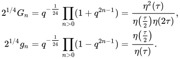
Siguiendo empleando el nombre , defina las funciones G y g de Ramanujan como q = e π i τ {\displaystyle q=e^{\pi i\tau }}

2 1 / 4 G n = q 1 24 n > 0 ( 1 + q 2 n 1 ) = η 2 ( τ ) η ( τ 2 ) η ( 2 τ ) , 2 1 / 4 g n = q 1 24 n > 0 ( 1 q 2 n 1 ) = η ( τ 2 ) η ( τ ) . {\displaystyle {\begin{aligned}2^{1/4}G_{n}&=q^{-{\frac {1}{24}}}\prod _{n>0}(1+q^{2n-1})={\frac {\eta ^{2}(\tau )}{\eta {\big (}{\tfrac {\tau }{2}}{\big )}\eta (2\tau )}},\\2^{1/4}g_{n}&=q^{-{\frac {1}{24}}}\prod _{n>0}(1-q^{2n-1})={\frac {\eta {\big (}{\tfrac {\tau }{2}}{\big )}}{\eta (\tau )}}.\end{aligned}}}

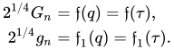
Los cocientes eta hacen que su conexión con las dos primeras funciones de Weber sea inmediatamente evidente. En el nome, supongamos que: τ = n . {\displaystyle \tau ={\sqrt {-n}}.}

2 1 / 4 G n = f ( q ) = f ( τ ) , 2 1 / 4 g n = f 1 ( q ) = f 1 ( τ ) . {\displaystyle {\begin{aligned}2^{1/4}G_{n}&={\mathfrak {f}}(q)={\mathfrak {f}}(\tau ),\\2^{1/4}g_{n}&={\mathfrak {f}}_{1}(q)={\mathfrak {f}}_{1}(\tau ).\end{aligned}}}

Ramanujan encontró muchas relaciones entre y que implican relaciones similares entre y . Por ejemplo, su identidad, G n {\displaystyle G_{n}} g n {\displaystyle g_{n}} f ( q ) {\displaystyle {\mathfrak {f}}(q)} f 1 ( q ) {\displaystyle {\mathfrak {f}}_{1}(q)}

( G n 8 g n 8 ) ( G n g n ) 8 = 1 4 , {\displaystyle (G_{n}^{8}-g_{n}^{8})(G_{n}\,g_{n})^{8}={\tfrac {1}{4}},}

conduce a

[ f 8 ( q ) f 1 8 ( q ) ] [ f ( q ) f 1 ( q ) ] 8 = [ 2 ] 8 . {\displaystyle {\big [}{\mathfrak {f}}^{8}(q)-{\mathfrak {f}}_{1}^{8}(q){\big ]}{\big [}{\mathfrak {f}}(q)\,{\mathfrak {f}}_{1}(q){\big ]}^{8}={\big [}{\sqrt {2}}{\big ]}^{8}.}

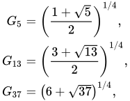
Para muchos valores de n , Ramanujan también tabuló para n impar y para n par . Esto automáticamente da muchas evaluaciones explícitas de y . Por ejemplo, utilizando , que son algunos de los discriminantes libres de cuadrados con número de clase 2, G n {\displaystyle G_{n}} g n {\displaystyle g_{n}} f ( q ) {\displaystyle {\mathfrak {f}}(q)} f 1 ( q ) {\displaystyle {\mathfrak {f}}_{1}(q)} τ = 5 , 13 , 37 {\displaystyle \tau ={\sqrt {-5}},\,{\sqrt {-13}},\,{\sqrt {-37}}}

G 5 = ( 1 + 5 2 ) 1 / 4 , G 13 = ( 3 + 13 2 ) 1 / 4 , G 37 = ( 6 + 37 ) 1 / 4 , {\displaystyle {\begin{aligned}G_{5}&=\left({\frac {1+{\sqrt {5}}}{2}}\right)^{1/4},\\G_{13}&=\left({\frac {3+{\sqrt {13}}}{2}}\right)^{1/4},\\G_{37}&=\left(6+{\sqrt {37}}\right)^{1/4},\end{aligned}}}

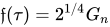
y uno puede obtener fácilmente de estos, así como de los ejemplos más complicados que se encuentran en los Cuadernos de Ramanujan. f ( τ ) = 2 1 / 4 G n {\displaystyle {\mathfrak {f}}(\tau )=2^{1/4}G_{n}}

Relación con las funciones theta de Jacobi

El argumento de las funciones theta clásicas de Jacobi es tradicionalmente el nome q = e π i τ , {\displaystyle q=e^{\pi i\tau },}

ϑ 10 ( 0 ; τ ) = θ 2 ( q ) = n = q ( n + 1 / 2 ) 2 = 2 η 2 ( 2 τ ) η ( τ ) , ϑ 00 ( 0 ; τ ) = θ 3 ( q ) = n = q n 2 = η 5 ( τ ) η 2 ( τ 2 ) η 2 ( 2 τ ) = η 2 ( τ + 1 2 ) η ( τ + 1 ) , ϑ 01 ( 0 ; τ ) = θ 4 ( q ) = n = ( 1 ) n q n 2 = η 2 ( τ 2 ) η ( τ ) . {\displaystyle {\begin{aligned}\vartheta _{10}(0;\tau )&=\theta _{2}(q)=\sum _{n=-\infty }^{\infty }q^{(n+1/2)^{2}}={\frac {2\eta ^{2}(2\tau )}{\eta (\tau )}},\\[2pt]\vartheta _{00}(0;\tau )&=\theta _{3}(q)=\sum _{n=-\infty }^{\infty }q^{n^{2}}\;=\;{\frac {\eta ^{5}(\tau )}{\eta ^{2}\left({\frac {\tau }{2}}\right)\eta ^{2}(2\tau )}}={\frac {\eta ^{2}\left({\frac {\tau +1}{2}}\right)}{\eta (\tau +1)}},\\[3pt]\vartheta _{01}(0;\tau )&=\theta _{4}(q)=\sum _{n=-\infty }^{\infty }(-1)^{n}q^{n^{2}}={\frac {\eta ^{2}\left({\frac {\tau }{2}}\right)}{\eta (\tau )}}.\end{aligned}}}

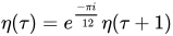
Dividiéndolos por , y también observando que , entonces son simplemente cuadrados de las funciones de Weber η ( τ ) {\displaystyle \eta (\tau )} η ( τ ) = e π i 12 η ( τ + 1 ) {\displaystyle \eta (\tau )=e^{\frac {-\pi i}{\,12}}\eta (\tau +1)} f i ( q ) {\displaystyle {\mathfrak {f}}_{i}(q)}

θ 2 ( q ) η ( τ ) = f 2 ( q ) 2 , θ 4 ( q ) η ( τ ) = f 1 ( q ) 2 , θ 3 ( q ) η ( τ ) = f ( q ) 2 , {\displaystyle {\begin{aligned}{\frac {\theta _{2}(q)}{\eta (\tau )}}&={\mathfrak {f}}_{2}(q)^{2},\\[4pt]{\frac {\theta _{4}(q)}{\eta (\tau )}}&={\mathfrak {f}}_{1}(q)^{2},\\[4pt]{\frac {\theta _{3}(q)}{\eta (\tau )}}&={\mathfrak {f}}(q)^{2},\end{aligned}}}

con funciones theta con subíndices pares enumeradas a propósito primero. Utilizando la conocida identidad de Jacobi con subíndices pares en el lado izquierdo,

θ 2 ( q ) 4 + θ 4 ( q ) 4 = θ 3 ( q ) 4 ; {\displaystyle \theta _{2}(q)^{4}+\theta _{4}(q)^{4}=\theta _{3}(q)^{4};}

por lo tanto,

f 2 ( q ) 8 + f 1 ( q ) 8 = f ( q ) 8 . {\displaystyle {\mathfrak {f}}_{2}(q)^{8}+{\mathfrak {f}}_{1}(q)^{8}={\mathfrak {f}}(q)^{8}.}

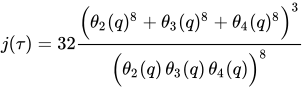
Relación con la función j

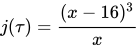
Las tres raíces de la ecuación cúbica

j ( τ ) = ( x 16 ) 3 x {\displaystyle j(\tau )={\frac {(x-16)^{3}}{x}}}

donde j ( τ ) es la función j y se expresan mediante . Además, dado que, x i = f ( τ ) 24 , f 1 ( τ ) 24 , f 2 ( τ ) 24 {\displaystyle x_{i}={\mathfrak {f}}(\tau )^{24},-{\mathfrak {f}}_{1}(\tau )^{24},-{\mathfrak {f}}_{2}(\tau )^{24}}

j ( τ ) = 32 ( θ 2 ( q ) 8 + θ 3 ( q ) 8 + θ 4 ( q ) 8 ) 3 ( θ 2 ( q ) θ 3 ( q ) θ 4 ( q ) ) 8 {\displaystyle j(\tau )=32{\frac {{\Big (}\theta _{2}(q)^{8}+\theta _{3}(q)^{8}+\theta _{4}(q)^{8}{\Big )}^{3}}{{\Big (}\theta _{2}(q)\,\theta _{3}(q)\,\theta _{4}(q){\Big )}^{8}}}}

y utilizando las definiciones de las funciones de Weber en términos de las funciones theta de Jacobi, más el hecho de que , entonces f 2 ( q ) 2 f 1 ( q ) 2 f ( q ) 2 = θ 2 ( q ) η ( τ ) θ 4 ( q ) η ( τ ) θ 3 ( q ) η ( τ ) = 2 {\displaystyle {\mathfrak {f}}_{2}(q)^{2}\,{\mathfrak {f}}_{1}(q)^{2}\,{\mathfrak {f}}(q)^{2}={\frac {\theta _{2}(q)}{\eta (\tau )}}{\frac {\theta _{4}(q)}{\eta (\tau )}}{\frac {\theta _{3}(q)}{\eta (\tau )}}=2}

j ( τ ) = ( f ( τ ) 16 + f 1 ( τ ) 16 + f 2 ( τ ) 16 2 ) 3 = ( f ( q ) 16 + f 1 ( q ) 16 + f 2 ( q ) 16 2 ) 3 {\displaystyle j(\tau )=\left({\frac {{\mathfrak {f}}(\tau )^{16}+{\mathfrak {f}}_{1}(\tau )^{16}+{\mathfrak {f}}_{2}(\tau )^{16}}{2}}\right)^{3}=\left({\frac {{\mathfrak {f}}(q)^{16}+{\mathfrak {f}}_{1}(q)^{16}+{\mathfrak {f}}_{2}(q)^{16}}{2}}\right)^{3}}

ya que y tienen las mismas fórmulas en términos de la función eta de Dedekind . f i ( τ ) = f i ( q ) {\displaystyle {\mathfrak {f}}_{i}(\tau )={\mathfrak {f}}_{i}(q)} η ( τ ) {\displaystyle \eta (\tau )}

Véase también

Referencias

  • Duke, William (2005), Fracciones continuas y funciones modulares (PDF) , Bull. Amer. Math. Soc. 42
  • Weber, Heinrich Martin (1981) [1898], Lehrbuch der Algebra (en alemán), vol. 3 (3.ª ed.), Nueva York: AMS Chelsea Publishing, ISBN 978-0-8218-2971-4
  • Yui, Noriko; Zagier, Don (1997), "Sobre los valores singulares de las funciones modulares de Weber", Mathematics of Computation , 66 (220): 1645–1662, doi : 10.1090/S0025-5718-97-00854-5 , MR  1415803

Notas

  1. ^ f , f 1 y f 2 no son funciones modulares (según la definición de Wikipedia), pero toda función modular es una función racional en f , f 1 y f 2 . Algunos autores utilizan una definición no equivalente de "funciones modulares".
  2. ^ https://www.math.ucla.edu/~wdduke/preprints/bams4.pdf Fracciones continuas y funciones modulares , W. Duke, págs. 22-23

Retrieved from "https://en.wikipedia.org/w/index.php?title=Weber_modular_function&oldid=1142265041"