Producto triple

Geométricamente, el triple producto escalar

${\displaystyle \mathbf {a} \cdot (\mathbf {b} \times \mathbf {c} )}$

es el volumen (con signo) del paralelepípedo definido por los tres vectores dados.

• El producto triple escalar no cambia bajo un desplazamiento circular de sus tres operandos ( a , b , c ):

  ${\displaystyle \mathbf {a} \cdot (\mathbf {b} \times \mathbf {c} )=\mathbf {b} \cdot (\mathbf {c} \times \mathbf {a} )=\mathbf {c} \cdot (\mathbf {a} \times \mathbf {b} )}$

• Intercambiar las posiciones de los operadores sin reordenar los operandos deja el producto triple sin cambios. Esto se deduce de la propiedad anterior y de la propiedad conmutativa del producto escalar:

  ${\displaystyle \mathbf {a} \cdot (\mathbf {b} \times \mathbf {c} )=(\mathbf {a} \times \mathbf {b} )\cdot \mathbf {c} }$

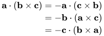
• Intercambiar dos cualesquiera de los tres operandos niega el producto triple. Esto se deduce de la propiedad de desplazamiento circular y de la anticonmutatividad del producto cruzado:

  ${\displaystyle {\begin{aligned}\mathbf {a} \cdot (\mathbf {b} \times \mathbf {c} )&=-\mathbf {a} \cdot (\mathbf {c} \times \mathbf {b} )\\&=-\mathbf {b} \cdot (\mathbf {a} \times \mathbf {c} )\\&=-\mathbf {c} \cdot (\mathbf {b} \times \mathbf {a} )\end{aligned}}}$

• El producto triple escalar también puede entenderse como el determinante de la matriz de 3 × 3 que tiene los tres vectores como filas o columnas (una matriz tiene el mismo determinante que su transpuesta ):

  ${\displaystyle \mathbf {a} \cdot (\mathbf {b} \times \mathbf {c} )=\det {\begin{bmatrix}a_{1}&a_{2}&a_{3}\\b_{1}&b_{2}&b_{3}\\c_{1}&c_{2}&c_{3}\\\end{bmatrix}}=\det {\begin{bmatrix}a_{1}&b_{1}&c_{1}\\a_{2}&b_{2}&c_{2}\\a_{3}&b_{3}&c_{3}\end{bmatrix}}=\det {\begin{bmatrix}\mathbf {a} &\mathbf {b} &\mathbf {c} \end{bmatrix}}.}$

• Si el producto triple escalar es igual a cero, entonces los tres vectores a , b y c son coplanares , ya que el paralelepípedo definido por ellos sería plano y no tendría volumen.
• Si dos vectores cualesquiera en el producto triple escalar son iguales, entonces su valor es cero:

  ${\displaystyle \mathbf {a} \cdot (\mathbf {a} \times \mathbf {b} )=\mathbf {a} \cdot (\mathbf {b} \times \mathbf {a} )=\mathbf {b} \cdot (\mathbf {a} \times \mathbf {a} )=0}$

• También:

  ${\displaystyle (\mathbf {a} \cdot (\mathbf {b} \times \mathbf {c} ))\,\mathbf {a} =(\mathbf {a} \times \mathbf {b} )\times (\mathbf {a} \times \mathbf {c} )}$

• El producto simple de dos productos triples (o el cuadrado de un producto triple) puede expandirse en términos de productos escalares: ^{[ 1 ]}$${\displaystyle ((\mathbf {a} \times \mathbf {b} )\cdot \mathbf {c} )\;((\mathbf {d} \times \mathbf {e} )\cdot \mathbf {f} )=\det {\begin{bmatrix}\mathbf {a} \cdot \mathbf {d} &\mathbf {a} \cdot \mathbf {e} &\mathbf {a} \cdot \mathbf {f} \\\mathbf {b} \cdot \mathbf {d} &\mathbf {b} \cdot \mathbf {e} &\mathbf {b} \cdot \mathbf {f} \\\mathbf {c} \cdot \mathbf {d} &\mathbf {c} \cdot \mathbf {e} &\mathbf {c} \cdot \mathbf {f} \end{bmatrix}}}$$Esto reformula en notación vectorial que el producto de los determinantes de dos matrices de 3 × 3 es igual al determinante de su producto matricial. Como caso especial, el cuadrado de un producto triple es un determinante de Gram . Nótese que este determinante está bien definido para vectores en R ^m ( espacio euclidiano m- dimensional ) incluso cuando m ≠ 3 ; en particular, el valor absoluto de un producto triple para tres vectores en R ^m se puede calcular a partir de esta fórmula para el cuadrado de un producto triple tomando su raíz cuadrada:$${\displaystyle |(\mathbf {a} \times \mathbf {b} )\cdot \mathbf {c} |={\sqrt {\det {\begin{bmatrix}\mathbf {a} \cdot \mathbf {a} &\mathbf {a} \cdot \mathbf {b} &\mathbf {a} \cdot \mathbf {c} \\\mathbf {b} \cdot \mathbf {a} &\mathbf {b} \cdot \mathbf {b} &\mathbf {b} \cdot \mathbf {c} \\\mathbf {c} \cdot \mathbf {a} &\mathbf {c} \cdot \mathbf {b} &\mathbf {c} \cdot \mathbf {c} \end{bmatrix}}}}}$$
• La razón entre el producto triple y el producto de las tres normas vectoriales se conoce como seno polar :$${\displaystyle {\frac {\mathbf {a} \cdot (\mathbf {b} \times \mathbf {c} )}{\left\|{\mathbf {a} }\right\|\left\|{\mathbf {b} }\right\|\left\|{\mathbf {c} }\right\|}}=\operatorname {psin} (\mathbf {a} ,\mathbf {b} ,\mathbf {c} )}$$que oscila entre -1 y 1.

En rigor, un escalar no cambia en absoluto bajo una transformación de coordenadas. (Por ejemplo, el factor de 2 utilizado para duplicar un vector no cambia si el vector está en coordenadas esféricas o rectangulares). Sin embargo, si cada vector se transforma mediante una matriz, el producto triple termina multiplicándose por el determinante de la matriz de transformación. Es decir, el producto triple de vectores covariantes se describe más apropiadamente como una densidad escalar .

$${\displaystyle {\begin{aligned}T\mathbf {a} \cdot (T\mathbf {b} \times T\mathbf {c} )&=\det {\begin{pmatrix}T\mathbf {a} &T\mathbf {b} &T\mathbf {c} \end{pmatrix}}\\&=\det \left(T{\begin{pmatrix}\mathbf {a} &\mathbf {b} &\mathbf {c} \end{pmatrix}}\right)\\&=\det(T)\det \!{\begin{pmatrix}\mathbf {a} &\mathbf {b} &\mathbf {c} \end{pmatrix}}\\&=\det(T)\left(\mathbf {a} \cdot (\mathbf {b} \times \mathbf {c} )\right)\end{aligned}}}$$

Algunos autores utilizan el término «pseudoescalar» para describir un objeto que se asemeja a un escalar, pero que no se transforma como tal. Dado que el producto triple se transforma como una densidad escalar y no como un escalar, podría denominarse «pseudoescalar» según esta definición más amplia. Sin embargo, el producto triple no es una «densidad pseudoescalar».

Cuando una transformación es una rotación que conserva la orientación, su determinante es +1 y el producto triple permanece inalterado. Cuando una transformación es una rotación que invierte la orientación, su determinante es −1 y el producto triple se niega. Una transformación arbitraria podría tener un determinante que no sea ni +1 ni −1 .

En álgebra exterior y álgebra geométrica, el producto exterior de dos vectores es un bivector , mientras que el producto exterior de tres vectores es un trivector . Un bivector es un elemento plano orientado y un trivector es un elemento volumétrico orientado, del mismo modo que un vector es un elemento lineal orientado.

Dados los vectores a , b y c , el producto

${\displaystyle \mathbf {a} \wedge \mathbf {b} \wedge \mathbf {c} }$

es un trivector con magnitud igual al producto triple escalar, es decir

${\displaystyle |\mathbf {a} \wedge \mathbf {b} \wedge \mathbf {c} |=|\mathbf {a} \cdot (\mathbf {b} \times \mathbf {c} )|}$,

y es el dual de Hodge del triple producto escalar. Como el producto exterior es asociativo, no se necesitan corchetes, ya que no importa cuál de a ∧ b o b ∧ c se calcule primero, aunque el orden de los vectores en el producto sí importa. Geométricamente, el trivector a ∧ b ∧ c corresponde al paralelepípedo generado por a , b y c , con los bivectores a ∧ b , b ∧ c y a ∧ c que coinciden con las caras paralelas del paralelepípedo.

El producto triple es idéntico a la forma de volumen del espacio euclidiano tridimensional aplicada a los vectores mediante el producto interior . También puede expresarse como una contracción de vectores con un tensor de rango 3 equivalente a la forma (o un pseudotensor equivalente a la pseudoforma de volumen); véase más abajo .

El${\displaystyle x}$componente de ${\displaystyle \mathbf {u} \times (\mathbf {v} \times \mathbf {w} )}$está dado por:

${\displaystyle {\begin{aligned}(\mathbf {u} \times (\mathbf {v} \times \mathbf {w} ))_{x}&=\mathbf {u} _{y}(\mathbf {v} _{x}\mathbf {w} _{y}-\mathbf {v} _{y}\mathbf {w} _{x})-\mathbf {u} _{z}(\mathbf {v} _{z}\mathbf {w} _{x}-\mathbf {v} _{x}\mathbf {w} _{z})\\&=\mathbf {v} _{x}(\mathbf {u} _{y}\mathbf {w} _{y}+\mathbf {u} _{z}\mathbf {w} _{z})-\mathbf {w} _{x}(\mathbf {u} _{y}\mathbf {v} _{y}+\mathbf {u} _{z}\mathbf {v} _{z})\\&=\mathbf {v} _{x}(\mathbf {u} _{y}\mathbf {w} _{y}+\mathbf {u} _{z}\mathbf {w} _{z})-\mathbf {w} _{x}(\mathbf {u} _{y}\mathbf {v} _{y}+\mathbf {u} _{z}\mathbf {v} _{z})+(\mathbf {u} _{x}\mathbf {v} _{x}\mathbf {w} _{x}-\mathbf {u} _{x}\mathbf {v} _{x}\mathbf {w} _{x})\\&=\mathbf {v} _{x}(\mathbf {u} _{x}\mathbf {w} _{x}+\mathbf {u} _{y}\mathbf {w} _{y}+\mathbf {u} _{z}\mathbf {w} _{z})-\mathbf {w} _{x}(\mathbf {u} _{x}\mathbf {v} _{x}+\mathbf {u} _{y}\mathbf {v} _{y}+\mathbf {u} _{z}\mathbf {v} _{z})\\&=(\mathbf {u} \cdot \mathbf {w} )\mathbf {v} _{x}-(\mathbf {u} \cdot \mathbf {v} )\mathbf {w} _{x}\end{aligned}}}$

De manera similar, el${\displaystyle y}$y${\displaystyle z}$componentes de ${\displaystyle \mathbf {u} \times (\mathbf {v} \times \mathbf {w} )}$son dados por:

${\displaystyle {\begin{aligned}(\mathbf {u} \times (\mathbf {v} \times \mathbf {w} ))_{y}&=(\mathbf {u} \cdot \mathbf {w} )\mathbf {v} _{y}-(\mathbf {u} \cdot \mathbf {v} )\mathbf {w} _{y}\\(\mathbf {u} \times (\mathbf {v} \times \mathbf {w} ))_{z}&=(\mathbf {u} \cdot \mathbf {w} )\mathbf {v} _{z}-(\mathbf {u} \cdot \mathbf {v} )\mathbf {w} _{z}\end{aligned}}}$

Al combinar estos tres componentes obtenemos:

${\displaystyle \mathbf {u} \times (\mathbf {v} \times \mathbf {w} )=(\mathbf {u} \cdot \mathbf {w} )\ \mathbf {v} -(\mathbf {u} \cdot \mathbf {v} )\ \mathbf {w} }$^{[ 5 ]}

Si se utiliza álgebra geométrica, el producto vectorial b × c de vectores se expresa como su producto exterior b ∧ c , un bivector . El segundo producto vectorial no puede expresarse como un producto exterior, ya que de lo contrario se obtendría el triple producto escalar. En su lugar, se puede utilizar una contracción izquierda ^{[ 6 ] , de modo que la fórmula se convierte en [ 7 ].}

${\displaystyle {\begin{aligned}-\mathbf {a} \;{\big \lrcorner }\;(\mathbf {b} \wedge \mathbf {c} )&=\mathbf {b} \wedge (\mathbf {a} \;{\big \lrcorner }\;\mathbf {c} )-(\mathbf {a} \;{\big \lrcorner }\;\mathbf {b} )\wedge \mathbf {c} \\&=(\mathbf {a} \cdot \mathbf {c} )\mathbf {b} -(\mathbf {a} \cdot \mathbf {b} )\mathbf {c} \end{aligned}}}$

La demostración se deriva de las propiedades de la contracción. ^{[ 6 ]} El resultado es el mismo vector que el calculado usando a × ( b × c ).

Utilizando los componentes individuales del producto cruzado

${\displaystyle \left(\mathbf {a} \times \mathbf {b} \right)_{\alpha }=\varepsilon _{\alpha \beta \gamma }a_{\beta }b_{\gamma }\,,}$

así como la expresión del símbolo Levi-Civita a través del delta de Kronecker

${\displaystyle \varepsilon _{\alpha \beta \gamma }\varepsilon _{\gamma \mu \nu }=\delta _{\alpha \mu }\delta _{\beta \nu }-\delta _{\alpha \nu }\delta _{\beta \mu }\,,}$

recibimos la expresión

${\displaystyle {\begin{aligned}\left(\mathbf {\hat {a}} \times \left(\mathbf {\hat {b}} \times \mathbf {\hat {c}} \right)\right)_{\alpha }&=\varepsilon _{\alpha \beta \gamma }{\hat {a}}_{\beta }\left(\mathbf {\hat {b}} \times \mathbf {\hat {c}} \right)_{\gamma }=\varepsilon _{\alpha \beta \gamma }{\hat {a}}_{\beta }\varepsilon _{\gamma \mu \nu }{\hat {b}}_{\mu }{\hat {c}}_{\nu }\\&=\left(\delta _{\alpha \mu }\delta _{\beta \nu }-\delta _{\alpha \nu }\delta _{\beta \mu }\right){\hat {a}}_{\beta }{\hat {b}}_{\mu }{\hat {c}}_{\nu }={\hat {a}}_{\beta }{\hat {b}}_{\alpha }{\hat {c}}_{\beta }-{\hat {a}}_{\beta }{\hat {b}}_{\beta }{\hat {c}}_{\alpha }\\&=\left({\hat {b}}_{\alpha }{\hat {a}}_{\beta }{\hat {c}}_{\beta }-{\hat {c}}_{\alpha }{\hat {a}}_{\beta }{\hat {b}}_{\beta }\right)+\left({\hat {a}}_{\beta }{\hat {b}}_{\alpha }{\hat {c}}_{\beta }-{\hat {b}}_{\alpha }{\hat {a}}_{\beta }{\hat {c}}_{\beta }\right)+\left({\hat {c}}_{\alpha }{\hat {a}}_{\beta }{\hat {b}}_{\beta }-{\hat {a}}_{\beta }{\hat {b}}_{\beta }{\hat {c}}_{\alpha }\right)\\&={\hat {b}}_{\alpha }\left({\hat {a}}_{\beta }{\hat {c}}_{\beta }\right)-{\hat {c}}_{\alpha }\left({\hat {a}}_{\beta }{\hat {b}}_{\beta }\right)+\left[{\hat {a}}_{\beta },{\hat {b}}_{\alpha }\right]{\hat {c}}_{\beta }+\left[{\hat {c}}_{\alpha },{\hat {a}}_{\beta }{\hat {b}}_{\beta }\right]\\&={\hat {b}}_{\alpha }\left(\mathbf {\hat {a}} \cdot \mathbf {\hat {c}} \right)-{\hat {c}}_{\alpha }\left(\mathbf {\hat {a}} \cdot \mathbf {\hat {b}} \right)+\left[{\hat {a}}_{\beta },{\hat {b}}_{\alpha }\right]{\hat {c}}_{\beta }+\left[{\hat {c}}_{\alpha },{\hat {a}}_{\beta }\right]{\hat {b}}_{\beta }+a_{\beta }\left[{\hat {c}}_{\alpha },{\hat {b}}_{\beta }\right]\end{aligned}}}$

para la primera identidad y la expresión

${\displaystyle {\begin{aligned}\left(\left(\mathbf {\hat {a}} \times \mathbf {\hat {b}} \right)\times \mathbf {\hat {c}} \right)_{\alpha }&=\varepsilon _{\alpha \beta \gamma }\left(\mathbf {\hat {a}} \times \mathbf {\hat {b}} \right)_{\beta }{\hat {c}}_{\gamma }=\varepsilon _{\alpha \beta \gamma }\varepsilon _{\beta \mu \nu }{\hat {a}}_{\mu }{\hat {b}}_{\nu }{\hat {c}}_{\gamma }\\&=\left(\delta _{\nu \alpha }\delta _{\mu \gamma }-\delta _{\mu \alpha }\delta _{\nu \gamma }\right){\hat {a}}_{\mu }{\hat {b}}_{\nu }{\hat {c}}_{\gamma }={\hat {a}}_{\mu }{\hat {b}}_{\alpha }{\hat {c}}_{\mu }-{\hat {a}}_{\alpha }{\hat {b}}_{\nu }{\hat {c}}_{\nu }\\&=\left({\hat {a}}_{\mu }{\hat {b}}_{\alpha }-{\hat {b}}_{\alpha }{\hat {a}}_{\mu }+{\hat {b}}_{\alpha }{\hat {a}}_{\mu }\right){\hat {c}}_{\mu }-{\hat {a}}_{\alpha }\left(\mathbf {\hat {b}} \cdot \mathbf {\hat {c}} \right)\\&=\left(\left[{\hat {a}}_{\mu },{\hat {b}}_{\alpha }\right]+{\hat {b}}_{\alpha }{\hat {a}}_{\mu }\right){\hat {c}}_{\mu }-{\hat {a}}_{\alpha }\left(\mathbf {\hat {b}} \cdot \mathbf {\hat {c}} \right)\\&={\hat {b}}_{\alpha }\left(\mathbf {\hat {a}} \cdot \mathbf {\hat {c}} \right)-{\hat {a}}_{\alpha }\left(\mathbf {\hat {b}} \cdot \mathbf {\hat {c}} \right)+\left[{\hat {a}}_{\mu },{\hat {b}}_{\alpha }\right]{\hat {c}}_{\mu }\end{aligned}}}$

para la segunda identidad para cada uno de los tres índices. Al expresarlos mediante una suma de todos los índices, se obtiene la identidad original.

Esta demostración se realiza tomando el dual de la versión de álgebra geométrica del producto vectorial triple hasta que todos los vectores se conviertan en bivectores.

${\displaystyle {\begin{alignedat}{3}&(-\mathbf {a} \;{\big \lrcorner }\;(\mathbf {b} \wedge \mathbf {c} ))\star &&=-{\tfrac {1}{2}}\left({\overset {\Rightarrow }{a}}(\mathbf {b} \wedge \mathbf {c} )-(\mathbf {b} \wedge \mathbf {c} ){\overset {\Rightarrow }{a}}\right)&&=-{\overset {\Rightarrow }{a}}\times (\mathbf {b} \wedge \mathbf {c} )\\&(-{\overset {\Rightarrow }{a}}\times (\mathbf {b} \wedge \mathbf {c} ))\star &&=-{\tfrac {1}{2}}\left({\overset {\Rightarrow }{a}}{\tfrac {1}{2}}({\overset {\Rightarrow }{b}}\mathbf {c} -\mathbf {c} {\overset {\Rightarrow }{b}})-{\tfrac {1}{2}}({\overset {\Rightarrow }{b}}\mathbf {c} -\mathbf {c} {\overset {\Rightarrow }{b}}){\overset {\Rightarrow }{a}}\right)&&=-{\overset {\Rightarrow }{a}}\times ({\overset {\Rightarrow }{b}}\cdot \mathbf {c} )\\&(-{\overset {\Rightarrow }{a}}\times ({\overset {\Rightarrow }{b}}\cdot \mathbf {c} ))\star &&=-{\tfrac {1}{2}}\left({\overset {\Rightarrow }{a}}{\tfrac {1}{2}}({\overset {\Rightarrow }{b}}{\overset {\Rightarrow }{c}}-{\overset {\Rightarrow }{c}}{\overset {\Rightarrow }{b}})-{\tfrac {1}{2}}({\overset {\Rightarrow }{b}}{\overset {\Rightarrow }{c}}-{\overset {\Rightarrow }{c}}{\overset {\Rightarrow }{b}}){\overset {\Rightarrow }{a}}\right)&&={\overset {\Rightarrow }{a}}\times ({\overset {\Rightarrow }{b}}\times {\overset {\Rightarrow }{c}})\end{alignedat}}}$

Fueron tres duelos. Esto también debe hacerse hacia el lado izquierdo.

${\displaystyle {\begin{aligned}&((((\mathbf {a} \cdot \mathbf {c} )\mathbf {b} -(\mathbf {a} \cdot \mathbf {b} )\mathbf {c} )\star )\star )\star \\&={\tfrac {1}{2}}({\overset {\Rightarrow }{a}}{\overset {\Rightarrow }{c}}+{\overset {\Rightarrow }{c}}{\overset {\Rightarrow }{a}}){\overset {\Rightarrow }{b}}-{\tfrac {1}{2}}({\overset {\Rightarrow }{a}}{\overset {\Rightarrow }{b}}+{\overset {\Rightarrow }{b}}{\overset {\Rightarrow }{a}}){\overset {\Rightarrow }{c}}\\&=({\overset {\Rightarrow }{a}}\cdot {\overset {\Rightarrow }{c}}){\overset {\Rightarrow }{b}}+({\overset {\Rightarrow }{a}}\cdot {\overset {\Rightarrow }{b}}){\overset {\Rightarrow }{c}}\end{aligned}}}$

Al negar ambos lados obtenemos:

${\displaystyle {\overset {\Rightarrow }{a}}\times ({\overset {\Rightarrow }{b}}\times {\overset {\Rightarrow }{c}})=-({\overset {\Rightarrow }{a}}\cdot {\overset {\Rightarrow }{c}}){\overset {\Rightarrow }{b}}+({\overset {\Rightarrow }{a}}\cdot {\overset {\Rightarrow }{b}}){\overset {\Rightarrow }{c}}}$