En matemáticas, el producto de Khatri-Rao o producto de Kronecker por bloques de dos matrices particionadas A {\displaystyle \mathbf {A} } y B {\displaystyle \mathbf {B} } se de...
Hispanopedia WikiContenido en espanolLectura gratuita
en el que el bloque ij es el producto de Kronecker de tamaño m i p i × n j q j de los bloques correspondientes de A y B , suponiendo que el número de particiones de filas y columnas de ambas matrices es igual. El tamaño del producto es entonces (Σ i m i p i ) × (Σ j n j q j ) .
Por ejemplo, si A y B son ambas matrices particionadas de 2 × 2 , por ejemplo:
El producto de Kronecker por columnas de dos matrices es un caso especial del producto de Khatri-Rao, tal como se definió anteriormente, y también puede denominarse producto de Khatri-Rao. Este producto supone que las particiones de las matrices son sus columnas. En este caso, m 1 = m , p 1 = p , n = q y para cada j : n j = q j = 1 . El producto resultante es una matriz mp × n en la que cada columna es el producto de Kronecker de las columnas correspondientes de A y B. Utilizando las matrices de los ejemplos anteriores con las columnas particionadas:
de modo que:
Esta versión por columnas del producto de Khatri-Rao es útil en enfoques de álgebra lineal para el procesamiento analítico de datos [ 5 ] y en la optimización de la solución de problemas inversos que involucran una matriz diagonal. [ 6 ] [ 7 ]
En 1996 se propuso el producto Khatri-Rao por columnas para estimar los ángulos de llegada (AOA) y los retrasos de las señales multitrayecto [ 8 ] y las cuatro coordenadas de las fuentes de señales [ 9 ] en un conjunto de antenas digitales .
Esta operación matricial se denominó "producto de división de caras" de matrices [ 11 ] [ 13 ] o "producto de Khatri-Rao transpuesto". Este tipo de operación se basa en productos de Kronecker fila por fila de dos matrices. Utilizando las matrices de los ejemplos anteriores con las filas particionadas:
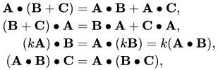
En las siguientes propiedades, el operadordenota el producto de Kronecker por filas (producto de división de caras) y el operadordenota el producto de Kronecker por columnas
El producto de división de caras por bloques transpuestos (o versión por columnas por bloques del producto de Khatri-Rao) de dos matrices particionadas con una cantidad dada de columnas en bloques tiene una vista: [ 9 ] [ 13 ]
El producto de división de caras y el producto de división de caras por bloques se utilizan en la teoría de matrices tensoriales de arreglos de antenas digitales . Estas operaciones también se utilizan en:
↑ Khatri CG, CR Rao (1968). "Soluciones a algunas ecuaciones funcionales y sus aplicaciones a la caracterización de distribuciones de probabilidad" . Sankhya . 30 : 167–180 . Archivado del original (PDF) el 23 de octubre de 2010. Consultado el 21 de agosto de 2008 .
↑ Liu, Shuangzhe (1999). "Resultados matriciales sobre los productos de Khatri-Rao y Tracy-Singh" . Álgebra lineal y sus aplicaciones . 289 ( 1–3 ): 267–277 . doi : 10.1016/S0024-3795(98)10209-4 .
↑ Zhang X; Yang Z; Cao C. (2002), "Desigualdades que involucran productos de Khatri-Rao de matrices semidefinidas positivas", Applied Mathematics E-notes , 2 : 117–124
↑ Liu, Shuangzhe; Trenkler, Götz (2008). "Hadamard, Khatri-Rao, Kronecker y otros productos matriciales". Revista Internacional de Ciencias de la Información y los Sistemas . 4 (1): 160– 177.
↑ Lev-Ari, Hanoch (1 de enero de 2005). "Solución eficiente de ecuaciones matriciales lineales con aplicación al procesamiento de conjuntos de antenas multiestáticas" (PDF) . Communications in Information and Systems . 05 (1): 123–130 . doi : 10.4310/CIS.2005.v5.n1.a5 . ISSN 1526-7555 .
↑ Vanderveen, MC, Ng, BC, Papadias, CB y Paulraj, A. (s.f.). Estimación conjunta de ángulo y retardo (JADE) para señales en entornos multitrayecto . Actas de la Trigésima Conferencia de Asilomar sobre Señales, Sistemas y Computadoras. – DOI:10.1109/acssc.1996.599145
^ Slyusar, VI ( 27 de diciembre de 1996 ) . "Productos de matriz final en aplicaciones de radar" (PDF) . Izvestiya VUZ: Radioelektronika . 41 (3): 71-75 .
↑ Anna Esteve, Eva Boj y Josep Fortiana (2009): "Términos de interacción en la regresión basada en distancias", Communications in Statistics – Theory and Methods , 38:19, pág. 3501
1 2 3 4 5 Slyusar, VI (1997-05-20). "Modelo analítico de la matriz de antenas digitales basado en productos de matrices de división de caras" (PDF) . Proc. ICATT-97, Kyiv : 108–109 .
1 2 3 4 5 6 7 8 Slyusar, VI (1997-09-15). "Nuevas operaciones de producto de matrices para aplicaciones de radares" (PDF) . Actas de Problemas Directos e Inversos de la Teoría de Ondas Electromagnéticas y Acústicas (DIPED-97), Lviv. : 73– 74.
1 2 3 4 5 6 7 8 9 10 Slyusar, VI (13 de marzo de 1998). "Una familia de productos de caras de matrices y sus propiedades" (PDF) . Cibernética y análisis de sistemas C/C de Kibernetika I Sistemnyi Analiz. 1999. 35 ( 3): 379– 384. doi : 10.1007/BF02733426 . S2CID 119661450 .
↑ Slyusar, VI (2003). "Productos faciales generalizados de matrices en modelos de conjuntos de antenas digitales con canales no idénticos" (PDF) . Radioelectronics and Communications Systems . 46 (10): 9– 17.
1 2 3 4 5 Vadym Slyusar. Nuevas operaciones matriciales para DSP (Conferencia). Abril de 1999. – DOI: 10.13140/RG.2.2.31620.76164/1
1 2 C. Radhakrishna Rao . Estimación de varianzas heterocedásticas en modelos lineales.//Journal of the American Statistical Association, vol. 65, n.º 329 (marzo de 1970), págs. 161-172
↑ Kasiviswanathan, Shiva Prasad, et al. «El precio de publicar tablas de contingencia de forma privada y los espectros de matrices aleatorias con filas correlacionadas». Actas del cuadragésimo segundo simposio de la ACM sobre teoría de la computación. 2010.
^ Thomas D. Ahle, Jakob Bæk Tejs Knudsen . Bosquejo tensorial casi óptimo. Publicado 2019. Matemáticas, Informática, ArXiv
↑ Ninh, Pham; Pagh, Rasmus (2013). Núcleos polinomiales rápidos y escalables mediante mapas de características explícitos . Conferencia internacional SIGKDD sobre descubrimiento de conocimiento y minería de datos. Association for Computing Machinery. doi : 10.1145/2487575.2487591 .
1 2 Eilers, Paul HC; Marx, Brian D. (2003). "Calibración multivariante con interacción de temperatura mediante regresión de señal penalizada bidimensional". Chemometrics and Intelligent Laboratory Systems . 66 (2): 159– 174. doi : 10.1016/S0169-7439(03)00029-7 .
1 2 3 Currie, ID; Durban, M.; Eilers, PHC (2006). "Modelos de matriz lineal generalizados con aplicaciones al suavizado multidimensional". Journal of the Royal Statistical Society . 68 (2): 259– 280. doi : 10.1111/j.1467-9868.2006.00543.x . S2CID 10261944 .
↑ Bryan Bischof. Tensores de coocurrencia de orden superior para hipergrafos mediante división de caras. Publicado el 15 de febrero de 2020, Matemáticas, Informática, ArXiv
↑ Johannes WR Martini, Jose Crossa, Fernando H. Toledo, Jaime Cuevas. Sobre los productos de Hadamard y Kronecker en estructuras de covarianza para la interacción genotipo x ambiente.//Plant Genome. 2020;13:e20033. Página 5.
Referencias
Khatri CG, CR Rao (1968). "Soluciones a algunas ecuaciones funcionales y sus aplicaciones a la caracterización de distribuciones de probabilidad" . Sankhya . 30 : 167–180 . Archivado del original el 23 de octubre de 2010. Recuperado el 21 de agosto de 2008 .
Rao CR; Rao M. Bhaskara (1998), Álgebra matricial y sus aplicaciones a la estadística y la econometría , World Scientific, pág. 216
Zhang X; Yang Z; Cao C. (2002), "Desigualdades que involucran productos de Khatri-Rao de matrices semidefinidas positivas", Applied Mathematics E-notes , 2 : 117–124
Liu Shuangzhe; Trenkler Götz ( 2008), "Hadamard, Khatri-Rao, Kronecker y otros productos matriciales", International Journal of Information and Systems Sciences , 4 : 160–177
 Hispanopedia Wiki


![{\displaystyle \mathbf {A} =\left[{\begin{array}{c | c}\mathbf {A} _{11}&\mathbf {A} _{12}\\\hline \mathbf {A} _{21}&\mathbf {A} _{22}\end{array}}\right]=\left[{\begin{array}{cc | c}1&2&3\\4&5&6\\\hline 7&8&9\end{array}}\right],\quad \mathbf {B} =\left[{\begin{array}{c | c}\mathbf {B} _{11}&\mathbf {B} _{12}\\\hline \mathbf {B} _{21}&\mathbf {B} _{22}\end{array}}\right]=\left[{\begin{array}{c | cc}1&4&7\\\hline 2&5&8\\3&6&9\end{array}}\right],}](https://wikimedia.org/api/rest_v1/media/math/render/svg/a53cde028551100b310943f25b2028a764436687)
![{\displaystyle \mathbf {A} \ast \mathbf {B} =\left[{\begin{array}{c | c}\mathbf {A} _{11}\otimes \mathbf {B} _{11}&\mathbf {A} _{12}\otimes \mathbf {B} _{12}\\\hline \mathbf {A} _{21}\otimes \mathbf {B} _{21}&\mathbf {A} _{22}\otimes \mathbf {B} _{22}\end{array}}\right]=\left[{\begin{array}{cc | cc}1&2&12&21\\4&5&24&42\\\hline 14&16&45&72\\21&24&54&81\end{array}}\right].}](https://wikimedia.org/api/rest_v1/media/math/render/svg/d2a086acf8812fc6ff3dec00cf40423b150b9942)
![{\displaystyle \mathbf {C} =\left[{\begin{array}{c | c | c}\mathbf {C} _{1}&\mathbf {C} _{2}&\mathbf {C} _{3}\end{array}}\right]=\left[{\begin{array}{c | c | c}1&2&3\\4&5&6\\7&8&9\end{array}}\right],\quad \mathbf {D} =\left[{\begin{array}{c | c | c }\mathbf {D} _{1}&\mathbf {D} _{2}&\mathbf {D} _{3}\end{array}}\right]=\left[{\begin{array}{c | c | c }1&4&7\\2&5&8\\3&6&9\end{array}}\right],}](https://wikimedia.org/api/rest_v1/media/math/render/svg/311fb96a2459096ea05d8f0461e67a8b49f5ee43)
![{\displaystyle \mathbf {C} \ast \mathbf {D} =\left[{\begin{array}{c | c | c }\mathbf {C} _{1}\otimes \mathbf {D} _{1}&\mathbf {C} _{2}\otimes \mathbf {D} _{2}&\mathbf {C} _{3}\otimes \mathbf {D} _{3}\end{array}}\right]=\left[{\begin{array}{c | c | c }1&8&21\\2&10&24\\3&12&27\\4&20&42\\8&25&48\\12&30&54\\7&32&63\\14&40&72\\21&48&81\end{array}}\right].}](https://wikimedia.org/api/rest_v1/media/math/render/svg/1e951f306d0dd52a9a56a35d767f2117db8a5ee6)
















![{\displaystyle (\mathbf {A} \otimes \mathbf {B} )\ast (\mathbf {C} \otimes \mathbf {D} )=\mathbf {P} [(\mathbf {A} \ast \mathbf {C} )\otimes (\mathbf {B} \ast \mathbf {D} )]}](https://wikimedia.org/api/rest_v1/media/math/render/svg/6b0be3bf1fc6226631d8af11b6bb868812171113)



















![{\displaystyle \mathbf {M} \bullet \mathbf {M} =\mathbf {M} [\circ ]\left(\mathbf {M} \otimes \mathbf {1} ^{\textsf {T}}\right)}](https://wikimedia.org/api/rest_v1/media/math/render/svg/a0ef70c0e73175eb22cda75ecb898d7779fb0441)
![{\displaystyle [\circ ]}](https://wikimedia.org/api/rest_v1/media/math/render/svg/9ae862b2ddef9fd1f7eb59ccec0f5f8ce6d30ae1)













![{\displaystyle {\begin{aligned}&\left({\begin{bmatrix}1&0\\0&1\\1&0\end{bmatrix}}\bullet {\begin{bmatrix}1&0\\1&0\\0&1\end{bmatrix}}\right)\left({\begin{bmatrix}1&1\\1&-1\end{bmatrix}}\otimes {\begin{bmatrix}1&1\\1&-1\end{bmatrix}}\right)\left({\begin{bmatrix}\sigma _{1}&0\\0&\sigma _{2}\\\end{bmatrix}}\otimes {\begin{bmatrix}\rho _{1}&0\\0&\rho _{2}\\\end{bmatrix}}\right)\left({\begin{bmatrix}x_{1}\\x_{2}\end{bmatrix}}\ast {\begin{bmatrix}y_{1}\\y_{2}\end{bmatrix}}\right)\\[5pt]{}={}&\left({\begin{bmatrix}1&0\\0&1\\1&0\end{bmatrix}}\bullet {\begin{bmatrix}1&0\\1&0\\0&1\end{bmatrix}}\right)\left({\begin{bmatrix}1&1\\1&-1\end{bmatrix}}{\begin{bmatrix}\sigma _{1}&0\\0&\sigma _{2}\\\end{bmatrix}}{\begin{bmatrix}x_{1}\\x_{2}\end{bmatrix}}\,\otimes \,{\begin{bmatrix}1&1\\1&-1\end{bmatrix}}{\begin{bmatrix}\rho _{1}&0\\0&\rho _{2}\\\end{bmatrix}}{\begin{bmatrix}y_{1}\\y_{2}\end{bmatrix}}\right)\\[5pt]{}={}&{\begin{bmatrix}1&0\\0&1\\1&0\end{bmatrix}}{\begin{bmatrix}1&1\\1&-1\end{bmatrix}}{\begin{bmatrix}\sigma _{1}&0\\0&\sigma _{2}\\\end{bmatrix}}{\begin{bmatrix}x_{1}\\x_{2}\end{bmatrix}}\,\circ \,{\begin{bmatrix}1&0\\1&0\\0&1\end{bmatrix}}{\begin{bmatrix}1&1\\1&-1\end{bmatrix}}{\begin{bmatrix}\rho _{1}&0\\0&\rho _{2}\\\end{bmatrix}}{\begin{bmatrix}y_{1}\\y_{2}\end{bmatrix}}.\end{aligned}}}](https://wikimedia.org/api/rest_v1/media/math/render/svg/077e2f2bb61c0f8393874c7f0ceb5f1bef78355c)



![{\displaystyle E\left[(T_{1}x)^{2}\right]=\left\|x\right\|_{2}^{2}}](https://wikimedia.org/api/rest_v1/media/math/render/svg/45663822e2a8c1b8b9b87a1a530b573089063f38)
![{\displaystyle E\left[(T_{1}x)^{p}\right]^{\frac {1}{p}}\leq {\sqrt {ap}}\|x\|_{2}}](https://wikimedia.org/api/rest_v1/media/math/render/svg/443c2d06bae7487f43814c4526a92bb3282cf0e8)









![{\displaystyle \mathbf {A} =\left[{\begin{array}{c | c}\mathbf {A} _{11}&\mathbf {A} _{12}\\\hline \mathbf {A} _{21}&\mathbf {A} _{22}\end{array}}\right],\quad \mathbf {B} =\left[{\begin{array}{c | c}\mathbf {B} _{11}&\mathbf {B} _{12}\\\hline \mathbf {B} _{21}&\mathbf {B} _{22}\end{array}}\right],}](https://wikimedia.org/api/rest_v1/media/math/render/svg/86b027efdf1b4ea7866bdc28bc7ac1b3809137bf)
![{\displaystyle \mathbf {A} [\bullet ]\mathbf {B} =\left[{\begin{array}{c | c}\mathbf {A} _{11}\bullet \mathbf {B} _{11}&\mathbf {A} _{12}\bullet \mathbf {B} _{12}\\\hline \mathbf {A} _{21}\bullet \mathbf {B} _{21}&\mathbf {A} _{22}\bullet \mathbf {B} _{22}\end{array}}\right].}](https://wikimedia.org/api/rest_v1/media/math/render/svg/8c5d6918b358808c418ec16679a5f86b9d93d4aa)
![{\displaystyle \mathbf {A} [\ast ]\mathbf {B} =\left[{\begin{array}{c | c}\mathbf {A} _{11}\ast \mathbf {B} _{11}&\mathbf {A} _{12}\ast \mathbf {B} _{12}\\\hline \mathbf {A} _{21}\ast \mathbf {B} _{21}&\mathbf {A} _{22}\ast \mathbf {B} _{22}\end{array}}\right].}](https://wikimedia.org/api/rest_v1/media/math/render/svg/1177613d963926bd03de425c42177de8661e5f55)
![{\displaystyle \left(\mathbf {A} [\ast ]\mathbf {B} \right)^{\textsf {T}}={\textbf {A}}^{\textsf {T}}[\bullet ]\mathbf {B} ^{\textsf {T}}}](https://wikimedia.org/api/rest_v1/media/math/render/svg/907ec4c862586658a29c538a04d6f973e129a19c)


