 Hispanopedia Wiki
En matemáticas , el teorema de inversión de Fourier establece que, para muchos tipos de funciones, es posible recuperar una función a partir de su transformada de Fourier . Intuitivamente, puede interpretarse como la afirmación de que, si conocemos toda la información de frecuencia y fase de una onda, podemos reconstruir la onda original con precisión.
El teorema dice que si tenemos una funciónque satisfacen ciertas condiciones, y utilizamos la convención para la transformada de Fourier que


entonces
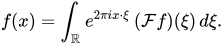
En otras palabras, el teorema dice que

Esta última ecuación se llama teorema integral de Fourier .
Otra forma de enunciar el teorema es que sies el operador de inversión, es decir, entonces



El teorema se cumple si ambosy su transformada de Fourier son absolutamente integrables (en el sentido de Lebesgue ) yes continua en el punto Sin embargo, incluso bajo condiciones más generales, se cumplen versiones del teorema de inversión de Fourier. En estos casos, las integrales anteriores pueden no converger en el sentido ordinario.


Declaración
En esta sección asumimos quees una función continua integrable . Utilice la convención para la transformada de Fourier que

Además, suponemos que la transformada de Fourier también es integrable.
Transformada inversa de Fourier como una integral
La formulación más común del teorema de inversión de Fourier es expresar la transformada inversa como una integral. Para cualquier función integrabley todocolocar


Entonces para todostenemos

Teorema integral de Fourier
El teorema puede reformularse como

Tomando la parte real [ 1 ] de cada lado de la expresión anterior obtenemos

Transformación inversa en términos del operador de inversión
Para cualquier funcióndefinir el operador de volteo [ 2 ]por

Entonces podemos definir en su lugar

Es inmediato a partir de la definición de la transformada de Fourier y del operador de inversión que ambosycoincidir con la definición integral de , y en particular son iguales entre sí y satisfacen .



Desdetenemosy.


Inverso bilateral
La forma del teorema de inversión de Fourier enunciado anteriormente, como es común, es que
En otras palabras,es una inversa izquierda de la transformada de Fourier. Sin embargo, también es una inversa derecha de la transformada de Fourier, es decir


Desdees tan similar a , esto se deduce muy fácilmente del teorema de inversión de Fourier (cambio de variables :=-\xi } ):


![{\displaystyle {\begin{aligned}f&={\mathcal {F}}^{-1}({\mathcal {F}}f)(x)\\[6pt]&=\int _{\mathbb {R} }\int _{\mathbb {R} }e^{2\pi ix\cdot \xi }\,e^{-2\pi iy\cdot \xi }\,f(y)\,dy\,d\xi \\[6pt]&=\int _{\mathbb {R} }\int _{\mathbb {R} }e^{-2\pi ix\cdot \zeta }\,e^{2\pi iy\cdot \zeta }\,f(y)\,dy\,d\zeta \\[6pt]&={\mathcal {F}}({\mathcal {F}}^{-1}f)(x).\end{aligned}}}](https://wikimedia.org/api/rest_v1/media/math/render/svg/2a07df5c4e14119ddb3c4b62067b107a0915efc8)
Alternativamente, esto se puede ver a partir de la relación entrey el operador de inversión y la asociatividad de la composición de funciones , ya que

Condiciones de funcionamiento
En física e ingeniería, el teorema de inversión de Fourier se suele utilizar bajo el supuesto de que todo se comporta de forma predecible. En matemáticas, este tipo de argumentos heurísticos no están permitidos, y el teorema de inversión de Fourier incluye una especificación explícita de la clase de funciones que admite. Sin embargo, no existe una clase de funciones "óptima", por lo que existen varias variantes del teorema de inversión de Fourier, aunque con conclusiones compatibles.
Funciones de Schwartz
El teorema de inversión de Fourier se cumple para todas las funciones de Schwartz (en términos generales, funciones suaves que decaen rápidamente y cuyas derivadas de cualquier orden también decaen rápidamente). Esta condición tiene la ventaja de ser una afirmación directa y elemental sobre la función (en lugar de imponer una condición a su transformada de Fourier), y la integral que define la transformada de Fourier y su inversa son absolutamente integrables. Esta versión del teorema se utiliza en la demostración del teorema de inversión de Fourier para distribuciones temperadas (véase más adelante).
Funciones integrables con transformada de Fourier integrable
El teorema de inversión de Fourier se cumple para todas las funciones continuas que son absolutamente integrables (es decir , ) con transformada de Fourier absolutamente integrable. Esto incluye todas las funciones de Schwartz, por lo que es una forma estrictamente más fuerte del teorema que la mencionada anteriormente. Esta condición es la que se utiliza arriba en la sección de enunciados .

Una ligera variante consiste en eliminar la condición de que la funciónser continua pero aún así requerir que tanto ella como su transformada de Fourier sean absolutamente integrables. Entoncescasi en todas partes donde g es una función continua, ypor cada.


Funciones integrables en una dimensión
- Suave por partes; una dimensión
Si la función es absolutamente integrable en una dimensión (es decir , ) y es suave por partes, entonces se cumple una versión del teorema de inversión de Fourier. En este caso definimos


Entonces para todos

es decires igual al promedio de los límites izquierdo y derecho deen . En los puntos dondees continuo esto simplemente es igual a.
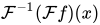

También se cumple una analogía de dimensiones superiores de esta forma del teorema, pero según Folland (1992) es "bastante delicada y no muy útil".
- Continuo por partes; una dimensión
Si la función es absolutamente integrable en una dimensión (es decir , ) pero simplemente continua por partes entonces una versión del teorema de inversión de Fourier sigue siendo válida. En este caso, la integral en la transformada inversa de Fourier se define con la ayuda de una función de corte suave en lugar de una función de corte abrupta; específicamente definimos

La conclusión del teorema es, por lo tanto, la misma que para el caso de funciones suaves por partes que se analizó anteriormente.
- Continuo; cualquier número de dimensiones
Sies continuo y absolutamente integrable enentonces el teorema de inversión de Fourier sigue siendo válido siempre que definamos nuevamente la transformada inversa con una función de corte suave, es decir


La conclusión ahora es simplemente que para todos
- Sin condición de regularidad; cualquier número de dimensiones
Si dejamos de lado todas las suposiciones sobre la continuidad (por partes) dey supongamos simplemente que es absolutamente integrable, entonces una versión del teorema sigue siendo válida. La transformada inversa se define de nuevo con el corte suave, pero con la conclusión de que
for almost every.
Square-integrable functions
In this case the Fourier transform cannot be defined directly as an integral since it may not be absolutely convergent, so it is instead defined by a density argument (see Fourier transform § On Lp spaces). For example, putting

we can set where the limit is taken in the -norm. The inverse transform may be defined by density in the same way or by defining it in terms of the Fourier transform and the flip operator. We then have



in the mean squared norm. In one dimension (and one dimension only), it can also be shown that it converges for almost every. This is Carleson's theorem, but is much harder to prove than convergence in the mean squared norm.
Tempered distributions
The Fourier transform may be defined on the space of tempered distributions by duality of the Fourier transform on the space of Schwartz functions. Specifically for and for all test functions we set


- :=\langle f,{\mathcal {F}}\varphi \rangle ,}

where is defined using the integral formula.[3] If then this agrees with the usual definition. We may define the inverse transform , either by duality from the inverse transform on Schwartz functions in the same way, or by defining it in terms of the flip operator (where the flip operator is defined by duality). We then have




Relation to Fourier series
The Fourier inversion theorem is analogous to the convergence of Fourier series. In the Fourier transform case we have


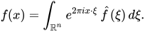
In the Fourier series case we instead have
![{\displaystyle f:[0,1]^{n}\to \mathbb {C} ,\quad {\hat {f}}:\mathbb {Z} ^{n}\to \mathbb {C} ,}](https://wikimedia.org/api/rest_v1/media/math/render/svg/5e2adf5138859dec7e350183a9d4ffc7b565142b)
![{\displaystyle {\hat {f}}(k):=\int _{[0,1]^{n}}e^{-2\pi iy\cdot k}\,f(y)\,dy,}](https://wikimedia.org/api/rest_v1/media/math/render/svg/7fbacfb859d551e558f0358273ca1598d6c7e064)
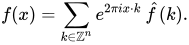
In particular, in one dimension and the sum runs from to .


Applications

In applications of the Fourier transform the Fourier inversion theorem often plays a critical role. In many situations the basic strategy is to apply the Fourier transform, perform some operation or simplification, and then apply the inverse Fourier transform.
More abstractly, the Fourier inversion theorem is a statement about the Fourier transform as an operator (see Fourier transform § Fourier transform on function spaces). For example, the Fourier inversion theorem on shows that the Fourier transform is a unitary operator on .


See also
Notes
- ↑w.l.o.g., f is real-valued, as any complex-valued function can be split into its real and imaginary parts and every operator appearing here is linear in f.
- ↑An operator is a transformation that maps functions to functions. The flip operator, the Fourier transform, the inverse Fourier transform and the identity transform are all examples of operators.
- ↑Folland 1992, p. 333.
References
- Folland, Gerald B. (1992). Fourier analysis and its applications. Pacific Grove, Calif: Wadsworth & Brooks/Cole. ISBN 978-0-534-17094-3.
- Folland, G. B. (1995). Introduction to Partial Differential Equations (2nd ed.). Princeton, USA: Princeton Univ. Press. ISBN 978-0-691-04361-6.
- Generalized functions
- Theorems in Fourier analysis
- Schwartz distributions