La notación de flechas encadenadas de Conway , creada por el matemático John Horton Conway , es un medio para expresar ciertos números extremadamente grandes . [1] Es simplemente una secuencia finita de números enteros positivos separados por flechas hacia la derecha, por ejemplo .
2 → 3 → 4 → 5 → 6
{\displaystyle 2\a 3\a 4\a 5\a 6}
Como ocurre con la mayoría de las notaciones combinatorias , la definición es recursiva . En este caso, la notación finalmente se resuelve como el número más a la izquierda elevado a una potencia entera (normalmente enorme).
Definición y descripción general Una "cadena Conway" se define de la siguiente manera:
Cualquier número entero positivo es una cadena de longitud .
1
{\estilo de visualización 1}
Una cadena de longitud n , seguida de una flecha hacia la derecha → y un entero positivo, juntos forman una cadena de longitud .
norte + 1
{\estilo de visualización n+1}
Cualquier cadena representa un número entero, según las seis reglas que se indican a continuación. Se dice que dos cadenas son equivalentes si representan el mismo número entero.
Sea n los números enteros positivos y sea n el resto inalterado de la cadena. Entonces:
a , b , do
{\estilo de visualización a,b,c}
#
{\estilo de visualización \#}
Una cadena vacía (o una cadena de longitud 0) es igual a
1
{\estilo de visualización 1}
La cadena representa el número .
a
{\estilo de visualización a}
a
{\estilo de visualización a}
La cadena representa el número .
a → b
{\displaystyle a\flecha derecha b}
a
b
Estilo de visualización a^{b}}
La cadena representa el número (ver la notación de flecha hacia arriba de Knuth )
a → b → do
{\displaystyle a\rightarrow b\rightarrow c}
a
↑
do
b
{\displaystyle a\uparrow ^{c}b}
Las cadenas y representan el mismo número que la cadena.
# → 1
{\displaystyle \#\rightarrow 1}
# → 1 → a
{\displaystyle \#\rightarrow 1\rightarrow a}
#
{\estilo de visualización \#}
De lo contrario, la cadena representa el mismo número que la cadena .
# → ( a + 1 ) → ( b + 1 )
{\displaystyle \#\rightarrow (a+1)\rightarrow (b+1)}
# → ( # → a → ( b + 1 ) ) → b
{\displaystyle \#\rightarrow (\#\rightarrow a\rightarrow (b+1))\rightarrow b}
Propiedades Sea denotado subcadenas de longitud 1 o mayor.
incógnita , Y
{\estilo de visualización X, Y}
Una cadena se evalúa como una potencia perfecta de su primer número. Por lo tanto, es igual a
1 → Y
{\displaystyle 1\to Y}
1
{\estilo de visualización 1}
incógnita → 1 → Y
{\displaystyle X\a 1\a Y}
es equivalente a
incógnita
{\estilo de visualización X}
2 → 2 → Y
{\displaystyle 2\to 2\to Y}
es igual a
4
{\estilo de visualización 4}
incógnita → 2 → 2
{\displaystyle X\a 2\a 2}
es equivalente a
incógnita → ( incógnita )
{\displaystyle X\to (X)}
Interpretación Hay que tener cuidado de tratar una cadena de flechas como un todo . Las cadenas de flechas no describen la aplicación iterada de un operador binario. Mientras que las cadenas de otros símbolos infijos (p. ej. 3 + 4 + 5 + 6 + 7) a menudo se pueden considerar en fragmentos (p. ej. (3 + 4) + 5 + (6 + 7)) sin un cambio de significado (véase asociatividad ), o al menos se pueden evaluar paso a paso en un orden prescrito, p. ej. 3 4 5 6 7 de derecha a izquierda, no ocurre lo mismo con las cadenas de flechas de Conway.
Por ejemplo:
2 → 3 → 2 = 2 ↑ ↑ 3 =
2
2
2
=
2
4
= 16
{\displaystyle 2\rightarrow 3\rightarrow 2=2\uparrow \uparrow 3=2^{2^{2}}=2^{4}=16}
2 → ( 3 → 2 ) =
2
3
2
=
2
9
= 512
{\displaystyle 2\rightarrow (3\rightarrow 2)=2^{3^{2}}=2^{9}=512}
( 2 → 3 ) → 2 = (
2
3
)
2
=
8
2
= 64
{\displaystyle (2\rightarrow 3)\rightarrow 2=(2^{3})^{2}=8^{2}=64}
La sexta regla de definición es la clave: una cadena de 4 o más elementos que termina en 2 o más se convierte en una cadena de la misma longitud con un penúltimo elemento (normalmente mucho) aumentado. Pero su último elemento se reduce, lo que finalmente permite que la quinta regla acorte la cadena. Después de, parafraseando a Knuth , "mucho detalle", la cadena se reduce a tres elementos y la cuarta regla termina la recursión.
Ejemplos Los ejemplos se complican rápidamente. A continuación se muestran algunos ejemplos pequeños:
norte
{\estilo de visualización n}
= norte
{\estilo de visualización =n}
(Por regla 2)
pag → q
{\displaystyle p\to q}
=
pag
q
{\displaystyle =p^{q}}
(Por la regla 3) De este modo,
3 → 4 =
3
4
= 81
{\displaystyle 3\a 4=3^{4}=81}
4 → 3 → 2
{\displaystyle 4\a 3\a 2}
= 4 ↑ ↑ 3
{\displaystyle =4\flecha arriba \flecha arriba 3}
(Por la regla 4)
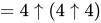
= 4 ↑ ( 4 ↑ 4 )
{\displaystyle =4\flecha arriba (4\flecha arriba 4)}
= 4 ↑ 256
{\displaystyle =4\flecha arriba 256}
=
4
256
{\estilo de visualización = 4^{256}}
= 13 , 407 , 807 , 929 , 942 , 597 , 099 , 574 , 024 , 998 , 205 , 846 , 127 , 479 , 365 , 820 , 592 , 393 , 377 , 723 , 561 , 443 , 721 , 764 , 030 , 073 ,
{\displaystyle =13,407,807,929,942,597,099,574,024,998,205,846,127,479,365,820,592,393,377,723,561,443,721,764,030,073,}
546 , 976 , 801 , 874 , 298 , 166 , 903 , 427 , 690 , 031 , 858 , 186 , 486 , 050 , 853 , 753 , 882 , 811 , 946 , 569 , 946 , 433 , 649 , 006 , 084 , 096
{\displaystyle 546,976,801,874,298,166,903,427,690,031,858,186,486,050,853,753,882,811,946,569,946,433,649,006,084,096}
≈ 1.34 ∗
10
154
{\displaystyle \aproximadamente 1,34*10^{154}}
2 → 2 → a
{\displaystyle 2\a 2\a a}
= 2 [
↑
a
] 2
{\displaystyle =2[\uparrow ^{a}]2}
(Por la regla 4)
= 4
{\estilo de visualización = 4}
(ver la notación de flecha hacia arriba de Knuth )
2 → 4 → 3
{\displaystyle 2\a 4\a 3}
= 2 ↑ ↑ ↑ 4
{\displaystyle =2\flecha arriba \flecha arriba \flecha arriba 4}
(Por la regla 4)
= 2 ↑ ↑ 2 ↑ ↑ 2 ↑ ↑ 2
{\displaystyle =2\flecha arriba \flecha arriba 2\flecha arriba \flecha arriba 2\flecha arriba \flecha arriba 2}
= 2 ↑ ↑ 2 ↑ ↑ 4
{\displaystyle =2\flecha arriba \flecha arriba 2\flecha arriba \flecha arriba 4}
= 2 ↑ ↑ 2 ↑ 2 ↑ 2 ↑ 2
{\displaystyle =2\flecha arriba \flecha arriba 2\flecha arriba 2\flecha arriba 2\flecha arriba 2}
= 2 ↑ ↑ 2 ↑ 2 ↑ 4
{\displaystyle =2\flecha arriba \flecha arriba 2\flecha arriba 2\flecha arriba 4}
= 2 ↑ ↑ 2 ↑ 16
{\displaystyle =2\flecha arriba \flecha arriba 2\flecha arriba 16}
= 2 ↑ ↑ 65536
{\displaystyle =2\flecha arriba \flecha arriba 65536}
=
65536
2
{\displaystyle ={^{65536}2}}
(ver tetración )
2 → 3 → 2 → 2
{\displaystyle 2\a 3\a 2\a 2}
= 2 → 3 → ( 2 → 3 ) → 1
{\displaystyle =2\a 3\a (2\a 3)\a 1}
(Por la regla 6)
= 2 → 3 → 8 → 1
{\displaystyle =2\a 3\a 8\a 1}
(Por la regla 3)
= 2 → 3 → 8
{\displaystyle =2\a 3\a 8}
(Por la regla 5)
= 2 → ( 2 → 2 → 8 ) → 7
{\displaystyle =2\a (2\a 2\a 8)\a 7}
(Por la regla 6)
= 2 → 4 → 7
{\displaystyle =2\a 4\a 7}
(Por la regla 6)
= 2 ↑↑↑↑↑↑↑
4
{\displaystyle =2\uparrow \uparrow \uparrow \uparrow \uparrow \uparrow \uparrow 4}
(Por la regla 4) = mucho mayor que el número anterior
3
→
2
→
2
→
2
{\displaystyle 3\to 2\to 2\to 2}
=
3
→
2
→
(
3
→
2
)
→
1
{\displaystyle =3\to 2\to (3\to 2)\to 1}
(Por la regla 6)
=
3
→
2
→
9
→
1
{\displaystyle =3\to 2\to 9\to 1}
(Por la regla 3)
=
3
→
2
→
9
{\displaystyle =3\to 2\to 9}
(Por la regla 5)
=
3
→
3
→
8
{\displaystyle =3\to 3\to 8}
(Por la regla 6)
=
3
↑↑↑↑↑↑↑↑
3
{\displaystyle =3\uparrow \uparrow \uparrow \uparrow \uparrow \uparrow \uparrow \uparrow 3}
(Por la regla 4) = mucho, mucho más grande que el número anterior
Ejemplos sistemáticos Los casos más simples con cuatro términos (que no contienen ningún número entero menor que 2) son:
a
→
b
→
2
→
2
{\displaystyle a\to b\to 2\to 2}
=
a
→
b
→
2
→
(
1
+
1
)
{\displaystyle =a\to b\to 2\to (1+1)}
=
a
→
b
→
(
a
→
b
)
→
1
{\displaystyle =a\to b\to (a\to b)\to 1}
=
a
→
b
→
a
b
{\displaystyle =a\to b\to a^{b}}
=
a
[
a
b
+
2
]
b
{\displaystyle =a[a^{b}+2]b}
(equivalente a la última propiedad mencionada)
a
→
b
→
3
→
2
{\displaystyle a\to b\to 3\to 2}
=
a
→
b
→
3
→
(
1
+
1
)
{\displaystyle =a\to b\to 3\to (1+1)}
=
a
→
b
→
(
a
→
b
→
(
a
→
b
)
→
1
)
→
1
{\displaystyle =a\to b\to (a\to b\to (a\to b)\to 1)\to 1}
=
a
→
b
→
(
a
→
b
→
a
b
)
{\displaystyle =a\to b\to (a\to b\to a^{b})}
=
a
[
a
→
b
→
2
→
2
+
2
]
b
{\displaystyle =a[a\to b\to 2\to 2+2]b}
a
→
b
→
4
→
2
{\displaystyle a\to b\to 4\to 2}
=
a
→
b
→
(
a
→
b
→
(
a
→
b
→
a
b
)
)
{\displaystyle =a\to b\to (a\to b\to (a\to b\to a^{b}))}
=
a
[
a
→
b
→
3
→
2
+
2
]
b
{\displaystyle =a[a\to b\to 3\to 2+2]b}
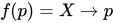
Podemos ver un patrón aquí. Si, para cualquier cadena , hacemos entonces (ver potencias funcionales ).
X
{\displaystyle X}
f
(
p
)
=
X
→
p
{\displaystyle f(p)=X\to p}
X
→
p
→
2
=
f
p
(
1
)
{\displaystyle X\to p\to 2=f^{p}(1)}
Aplicando esto con , entonces y
X
=
a
→
b
{\displaystyle X=a\to b}
f
(
p
)
=
a
[
p
+
2
]
b
{\displaystyle f(p)=a[p+2]b}
a
→
b
→
p
→
2
=
a
[
a
→
b
→
(
p
−
1
)
→
2
+
2
]
b
=
f
p
(
1
)
{\displaystyle a\to b\to p\to 2=a[a\to b\to (p-1)\to 2+2]b=f^{p}(1)}
Así, por ejemplo, .
10
→
6
→
3
→
2
=
10
[
10
[
1000002
]
6
+
2
]
6
{\displaystyle 10\to 6\to 3\to 2=10[10[1000002]6+2]6}
Siguiendo adelante:
a
→
b
→
2
→
3
{\displaystyle a\to b\to 2\to 3}
=
a
→
b
→
2
→
(
2
+
1
)
{\displaystyle =a\to b\to 2\to (2+1)}
=
a
→
b
→
(
a
→
b
)
→
2
{\displaystyle =a\to b\to (a\to b)\to 2}
=
a
→
b
→
a
b
→
2
{\displaystyle =a\to b\to a^{b}\to 2}
=
f
a
b
(
1
)
{\displaystyle =f^{a^{b}}(1)}
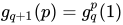
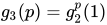
Nuevamente podemos generalizar. Cuando escribimos tenemos , es decir, . En el caso anterior, y , entonces
g
q
(
p
)
=
X
→
p
→
q
{\displaystyle g_{q}(p)=X\to p\to q}
X
→
p
→
q
+
1
=
g
q
p
(
1
)
{\displaystyle X\to p\to q+1=g_{q}^{p}(1)}
g
q
+
1
(
p
)
=
g
q
p
(
1
)
{\displaystyle g_{q+1}(p)=g_{q}^{p}(1)}
g
2
(
p
)
=
a
→
b
→
p
→
2
=
f
p
(
1
)
{\displaystyle g_{2}(p)=a\to b\to p\to 2=f^{p}(1)}
g
3
(
p
)
=
g
2
p
(
1
)
{\displaystyle g_{3}(p)=g_{2}^{p}(1)}
a
→
b
→
2
→
3
=
g
3
(
2
)
=
g
2
2
(
1
)
=
g
2
(
g
2
(
1
)
)
=
f
f
(
1
)
(
1
)
=
f
a
b
(
1
)
{\displaystyle a\to b\to 2\to 3=g_{3}(2)=g_{2}^{2}(1)=g_{2}(g_{2}(1))=f^{f(1)}(1)=f^{a^{b}}(1)}
Función de Ackermann La función de Ackermann se puede expresar utilizando la notación de flecha encadenada de Conway:
A
(
m
,
n
)
=
(
2
→
(
n
+
3
)
→
(
m
−
2
)
)
−
3
{\displaystyle A(m,n)=(2\to (n+3)\to (m-2))-3}
para (Ya que en hiperoperación )
m
≥
3
{\displaystyle m\geq 3}
A
(
m
,
n
)
=
2
[
m
]
(
n
+
3
)
−
3
{\displaystyle A(m,n)=2[m](n+3)-3}
por eso
2
→
n
→
m
=
A
(
m
+
2
,
n
−
3
)
+
3
{\displaystyle 2\to n\to m=A(m+2,n-3)+3}
para
n
>
2
{\displaystyle n>2}
( y correspondería con y , que lógicamente podrían añadirse).
n
=
1
{\displaystyle n=1}
n
=
2
{\displaystyle n=2}
A
(
m
,
−
2
)
=
−
1
{\displaystyle A(m,-2)=-1}
A
(
m
,
−
1
)
=
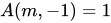
1
{\displaystyle A(m,-1)=1}
El número de Graham El número de Graham no se puede expresar en notación de flecha encadenada de Conway, pero está limitado por lo siguiente:
3
→
3
→
64
→
2
<
G
<
3
→
3
→
65
→
2
{\displaystyle 3\rightarrow 3\rightarrow 64\rightarrow 2<G<3\rightarrow 3\rightarrow 65\rightarrow 2}
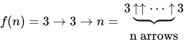
Demostración: primero definimos la función intermedia , que puede utilizarse para definir el número de Graham como . (El superíndice 64 denota una potencia funcional .)
f
(
n
)
=
3
→
3
→
n
=
3
↑↑
⋯
↑
⏟
3
n arrows
{\displaystyle f(n)=3\rightarrow 3\rightarrow n={\begin{matrix}3\underbrace {\uparrow \uparrow \cdots \uparrow } 3\\{\text{n arrows}}\end{matrix}}}
G
=
f
64
(
4
)
{\displaystyle G=f^{64}(4)}
Aplicando la regla 2 y la regla 4 al revés, simplificamos:
f
64
(
1
)
{\displaystyle f^{64}(1)}
=
3
→
3
→
(
3
→
3
→
(
⋯
(
3
→
3
→
(
3
→
3
→
1
)
)
⋯
)
)
{\displaystyle =3\rightarrow 3\rightarrow (3\rightarrow 3\rightarrow (\cdots (3\rightarrow 3\rightarrow (3\rightarrow 3\rightarrow 1))\cdots ))}
(con 64 's)
3
→
3
{\displaystyle 3\rightarrow 3}
=
3
→
3
→
(
3
→
3
→
(
⋯
(
3
→
3
→
(
3
→
3
)
→
1
)
⋯
)
→
1
)
→
1
{\displaystyle =3\rightarrow 3\rightarrow (3\rightarrow 3\rightarrow (\cdots (3\rightarrow 3\rightarrow (3\rightarrow 3)\rightarrow 1)\cdots )\rightarrow 1)\rightarrow 1}
=
3
→
3
→
64
→
2
;
{\displaystyle =3\rightarrow 3\rightarrow 64\rightarrow 2;}
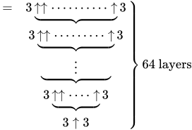
=
3
↑↑
⋯
⋯
⋯
⋅
↑
⏟
3
3
↑↑
⋯
⋯
⋯
↑
⏟
3
⋮
⏟
3
↑↑
⋯
⋅
↑
⏟
3
3
↑
3
}
64 layers
{\displaystyle \left.{\begin{matrix}=&3\underbrace {\uparrow \uparrow \cdots \cdots \cdots \cdot \uparrow } 3\\&3\underbrace {\uparrow \uparrow \cdots \cdots \cdots \uparrow } 3\\&\underbrace {\qquad \;\;\vdots \qquad \;\;} \\&3\underbrace {\uparrow \uparrow \cdots \cdot \uparrow } 3\\&3\uparrow 3\end{matrix}}\right\}{\text{64 layers}}}
f
64
(
4
)
=
G
;
{\displaystyle f^{64}(4)=G;}
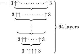
=
3
→
3
→
(
3
→
3
→
(
⋯
(
3
→
3
→
(
3
→
3
→
4
)
)
⋯
)
)
{\displaystyle =3\rightarrow 3\rightarrow (3\rightarrow 3\rightarrow (\cdots (3\rightarrow 3\rightarrow (3\rightarrow 3\rightarrow 4))\cdots ))}
(con 64 's)
3
→
3
{\displaystyle 3\rightarrow 3}
=
3
↑↑
⋯
⋯
⋯
⋅
↑
⏟
3
3
↑↑
⋯
⋯
⋯
↑
⏟
3
⋮
⏟
3
↑↑
⋯
⋅
↑
⏟
3
3
↑↑↑↑
3
}
64 layers
{\displaystyle \left.{\begin{matrix}=&3\underbrace {\uparrow \uparrow \cdots \cdots \cdots \cdot \uparrow } 3\\&3\underbrace {\uparrow \uparrow \cdots \cdots \cdots \uparrow } 3\\&\underbrace {\qquad \;\;\vdots \qquad \;\;} \\&3\underbrace {\uparrow \uparrow \cdots \cdot \uparrow } 3\\&3\uparrow \uparrow \uparrow \uparrow 3\end{matrix}}\right\}{\text{64 layers}}}
f
64
(
27
)
{\displaystyle f^{64}(27)}
=
3
→
3
→
(
3
→
3
→
(
⋯
(
3
→
3
→
(
3
→
3
→
27
)
)
⋯
)
)
{\displaystyle =3\rightarrow 3\rightarrow (3\rightarrow 3\rightarrow (\cdots (3\rightarrow 3\rightarrow (3\rightarrow 3\rightarrow 27))\cdots ))}
(con 64 's)
3
→
3
{\displaystyle 3\rightarrow 3}
=
3
→
3
→
(
3
→
3
→
(
⋯
(
3
→
3
→
(
3
→
3
→
(
3
→
3
)
)
)
⋯
)
)
{\displaystyle =3\rightarrow 3\rightarrow (3\rightarrow 3\rightarrow (\cdots (3\rightarrow 3\rightarrow (3\rightarrow 3\rightarrow (3\rightarrow 3)))\cdots ))}
(con 65 's)
3
→
3
{\displaystyle 3\rightarrow 3}
=
3
→
3
→
65
→
2
{\displaystyle =3\rightarrow 3\rightarrow 65\rightarrow 2}
(calculando como arriba).
=
f
65
(
1
)
{\displaystyle =f^{65}(1)}
=
3
↑↑
⋯
⋯
⋯
⋅
↑
⏟
3
3
↑↑
⋯
⋯
⋯
↑
⏟
3
⋮
⏟
3
↑↑
⋯
⋅
↑
⏟
3
3
↑
3
}
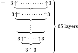
65 layers
{\displaystyle \left.{\begin{matrix}=&3\underbrace {\uparrow \uparrow \cdots \cdots \cdots \cdot \uparrow } 3\\&3\underbrace {\uparrow \uparrow \cdots \cdots \cdots \uparrow } 3\\&\underbrace {\qquad \;\;\vdots \qquad \;\;} \\&3\underbrace {\uparrow \uparrow \cdots \cdot \uparrow } 3\\&3\uparrow 3\end{matrix}}\right\}{\text{65 layers}}}
Dado que f es estrictamente creciente ,
f
64
(
1
)
<
f
64
(
4
)
<
f
64
(
27
)
{\displaystyle f^{64}(1)<f^{64}(4)<f^{64}(27)}
cual es la desigualdad dada.
Con flechas encadenadas, es muy fácil especificar un número mucho mayor que el número de Graham, por ejemplo, .
3
→
3
→
3
→
3
{\displaystyle 3\rightarrow 3\rightarrow 3\rightarrow 3}
3
→
3
→
3
→
3
{\displaystyle 3\rightarrow 3\rightarrow 3\rightarrow 3}
=
3
→
3
→
(
3
→
3
→
27
→
2
)
→
2
{\displaystyle =3\rightarrow 3\rightarrow (3\rightarrow 3\rightarrow 27\rightarrow 2)\rightarrow 2\,}
=
f
3
→
3
→
27
→
2
(
1
)
{\displaystyle =f^{3\rightarrow 3\rightarrow 27\rightarrow 2}(1)}
=
f
f
27
(
1
)
(
1
)
{\displaystyle =f^{f^{27}(1)}(1)}
=
3
↑↑
⋯
⋯
⋯
⋅
⋅
↑
⏟
3
3
↑↑
⋯
⋯
⋯
⋅
↑
⏟
3
3
↑↑
⋯
⋯
⋯
↑
⏟
3
⋮
⏟
3
↑↑
⋯
⋅
↑
⏟
3
3
↑
3
}
3
↑↑
⋯
⋯
⋯
⋅
↑
⏟
3
3
↑↑
⋯
⋯
⋯
↑
⏟
3
⋮
⏟
3
↑↑
⋯
⋅
↑
⏟
3
3
↑
3
}
27
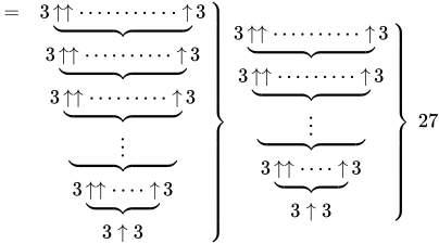
{\displaystyle \left.{\begin{matrix}=&3\underbrace {\uparrow \uparrow \cdots \cdots \cdots \cdot \cdot \uparrow } 3\\&3\underbrace {\uparrow \uparrow \cdots \cdots \cdots \cdot \uparrow } 3\\&3\underbrace {\uparrow \uparrow \cdots \cdots \cdots \uparrow } 3\\&\underbrace {\qquad \;\;\vdots \qquad \;\;} \\&3\underbrace {\uparrow \uparrow \cdots \cdot \uparrow } 3\\&3\uparrow 3\end{matrix}}\right\}\left.{\begin{matrix}3\underbrace {\uparrow \uparrow \cdots \cdots \cdots \cdot \uparrow } 3\\3\underbrace {\uparrow \uparrow \cdots \cdots \cdots \uparrow } 3\\\underbrace {\qquad \;\;\vdots \qquad \;\;} \\3\underbrace {\uparrow \uparrow \cdots \cdot \uparrow } 3\\3\uparrow 3\end{matrix}}\right\}\ 27}
que es mucho mayor que el número de Graham, porque el número es mucho mayor que .
3
→
3
→
27
→
2
{\displaystyle 3\rightarrow 3\rightarrow 27\rightarrow 2}
=
f
27
(
1
)
{\displaystyle =f^{27}(1)}
65
{\displaystyle 65}
Función CG Conway y Guy crearon una función simple de un solo argumento que diagonaliza sobre toda la notación, definida como:
c
g
(
n
)
=
n
→
n
→
n
→
⋯
→
n
→
n
→
n
⏟
n
{\displaystyle cg(n)=\underbrace {n\rightarrow n\rightarrow n\rightarrow \dots \rightarrow n\rightarrow n\rightarrow n} _{n}}
lo que significa que la secuencia es:
c
g
(
1
)
=
1
{\displaystyle cg(1)=1}
c
g
(
2
)
=
2
→
2
=
2
2
=
4
{\displaystyle cg(2)=2\to 2=2^{2}=4}
c
g
(
3
)
=
3
→
3
→
3
=
3
↑↑↑
3
{\displaystyle cg(3)=3\to 3\to 3=3\uparrow \uparrow \uparrow 3}
c
g
(
4
)
=
4
→
4
→
4
→
4
{\displaystyle cg(4)=4\to 4\to 4\to 4}
c
g
(
5
)
=
5
→
5
→
5
→
5
→
5
{\displaystyle cg(5)=5\to 5\to 5\to 5\to 5}
...
Esta función, como era de esperar, crece extraordinariamente rápido.
Ampliación de Peter Hurford Peter Hurford, desarrollador web y estadístico, ha definido una extensión de esta notación:
a
→
b
c
=
a
→
b
−
1
a
→
b
−
1
a
→
b
−
1
⋯
→
b
−
1
a
→
b
−
1
a
→
b
−
1
a
⏟
c
arrows
{\displaystyle a\rightarrow _{b}c=\underbrace {a\rightarrow _{b-1}a\rightarrow _{b-1}a\rightarrow _{b-1}\dots \rightarrow _{b-1}a\rightarrow _{b-1}a\rightarrow _{b-1}a} _{c{\text{ arrows}}}}
a
→
1
b
=
a
→
b
{\displaystyle a\rightarrow _{1}b=a\rightarrow b}
Por lo demás, todas las reglas normales no sufren modificaciones.
a
→
2
(
a
−
1
)
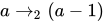
{\displaystyle a\rightarrow _{2}(a-1)}
ya es igual a la mencionada anteriormente , y la función crece mucho más rápido que la de Conway y Guy .
c
g
(
a
)
{\displaystyle cg(a)}
f
(
n
)
=
n
→
n
n
{\displaystyle f(n)=n\rightarrow _{n}n}
c
g
(
n
)
{\displaystyle cg(n)}
Tenga en cuenta que expresiones como son ilegales si y son números diferentes; una cadena debe tener solo un tipo de flecha hacia la derecha.
a
→
b
c
→
d
e
{\displaystyle a\rightarrow _{b}c\rightarrow _{d}e}
b
{\displaystyle b}
d
{\displaystyle d}
Sin embargo, si modificamos esto ligeramente de modo que:
a
→
b
c
→
d
e
=
a
→
b
c
→
d
−
1
c
→
d
−
1
c
→
d
−
1
⋯
→
d
−
1
c
→
d
−
1
c
→
d
−
1
c
⏟
e
arrows
{\displaystyle a\rightarrow _{b}c\rightarrow _{d}e=a\rightarrow _{b}\underbrace {c\rightarrow _{d-1}c\rightarrow _{d-1}c\rightarrow _{d-1}\dots \rightarrow _{d-1}c\rightarrow _{d-1}c\rightarrow _{d-1}c} _{e{\text{ arrows}}}}
Entonces no sólo se vuelve legal, sino que la notación en su conjunto se vuelve mucho más fuerte. [2]
a
→
b
c
→
d
e
{\displaystyle a\rightarrow _{b}c\rightarrow _{d}e}
Véase también
Referencias
^ John H. Conway y Richard K. Guy, El libro de los números, 1996, págs. 59-62 ^ "Números grandes, parte 2: Graham y Conway - Greatplay.net". archive.is . 2013-06-25. Archivado desde el original el 2013-06-25 . Consultado el 2018-02-18 .
Enlaces externos Factoides > números grandes Los grandes números de Robert Munafo El libro de los números de JH Conway y RK Guy
 Hispanopedia Wiki




















![{\displaystyle =2[\uparrow ^{a}]2}](https://wikimedia.org/api/rest_v1/media/math/render/svg/0852337ffde60d0eed6ca41e89526146604aef82)


























![{\displaystyle =a[a^{b}+2]b}](https://wikimedia.org/api/rest_v1/media/math/render/svg/5122c5c8b65604a751640ca32b6fa474637eaeec)




![{\displaystyle =a[a\a b\a 2\a 2+2]b}](https://wikimedia.org/api/rest_v1/media/math/render/svg/53ae38786c37933b56883d852a17a2b8e4f1d222)


![{\displaystyle =a[a\a b\a 3\a 2+2]b}](https://wikimedia.org/api/rest_v1/media/math/render/svg/41077be13272dbc2d9a89dd71889a505af53c6c1)


![{\displaystyle f(p)=a[p+2]b}](https://wikimedia.org/api/rest_v1/media/math/render/svg/8aa52d519ad9feefeac497887ca4f3174ea7fd80)
![{\displaystyle a\to b\to p\to 2=a[a\to b\to (p-1)\to 2+2]b=f^{p}(1)}](https://wikimedia.org/api/rest_v1/media/math/render/svg/8462b1d161e5a1235b8676f01d91a95614413f6c)
![{\displaystyle 10\a 6\a 3\a 2=10[10[1000002]6+2]6}](https://wikimedia.org/api/rest_v1/media/math/render/svg/394bc08c1e102d965a3ad763b59411596e67b264)











-3}](https://wikimedia.org/api/rest_v1/media/math/render/svg/22bbf4a6288580a0d9a85b22ca4cad21046ed3e6)