Vector aleatorio complejo

En teoría de probabilidad y estadística , un vector aleatorio complejo es típicamente una tupla de variables aleatorias de valor complejo y, en general, es una variable aleatoria que toma valores en un espacio vectorial sobre el cuerpo de números complejos. Si son variables aleatorias de valor complejo, entonces la n -tupla es un vector aleatorio complejo. Las variables aleatorias complejas siempre pueden considerarse como pares de vectores aleatorios reales: sus partes reales e imaginarias. ${\displaystyle Z_{1},\ldots,Z_{n}}$${\displaystyle \left(Z_{1},\ldots ,Z_{n}\right)}$

Algunos conceptos de vectores aleatorios reales tienen una generalización directa a los vectores aleatorios complejos. Por ejemplo, la definición de la media de un vector aleatorio complejo. Otros conceptos son exclusivos de los vectores aleatorios complejos.

Las aplicaciones de vectores aleatorios complejos se encuentran en el procesamiento de señales digitales .

Un vector aleatorio complejo en el espacio de probabilidad es una función tal que el vector es un vector aleatorio real en donde denota la parte real de y denota la parte imaginaria de . ^{[1] : p. 292}${\displaystyle \mathbf {Z} =(Z_{1},\ldots ,Z_{n})^{T}}$ ${\displaystyle (\Omega ,{\mathcal {F}},P)}$ ${\displaystyle \mathbf {Z} \colon \Omega \rightarrow \mathbb {C} ^{n}}$${\displaystyle (\Re {(Z_{1})},\Im {(Z_{1})},\ldots ,\Re {(Z_{n})},\Im {(Z_{n})})^{T}}$${\displaystyle (\Omega ,{\mathcal {F}},P)}$${\displaystyle \Re {(z)}}$${\displaystyle z}$${\displaystyle \Im {(z)}}$${\displaystyle z}$

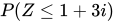
La generalización de la función de distribución acumulativa de variables aleatorias reales a complejas no es obvia porque las expresiones de la forma no tienen sentido. Sin embargo, las expresiones de la forma sí tienen sentido. Por lo tanto, la función de distribución acumulativa de un vector aleatorio se define como ${\displaystyle P(Z\leq 1+3i)}$${\displaystyle P(\Re {(Z)}\leq 1,\Im {(Z)}\leq 3)}$${\displaystyle F_{\mathbf {Z} }:\mathbb {C} ^{n}\mapsto [0,1]}$${\displaystyle \mathbf {Z} =(Z_{1},...,Z_{n})^{T}}$

dónde . ${\displaystyle \mathbf {z} =(z_{1},...,z_{n})^{T}}$

Como en el caso real, la expectativa (también llamada valor esperado ) de un vector aleatorio complejo se toma componente por componente. ^{[1] : p. 293}

La matriz de covarianza (también llamada segundo momento central ) contiene las covarianzas entre todos los pares de componentes. La matriz de covarianza de un vector aleatorio es una matriz cuyo elemento ⁿ es la covarianza entre la i ^ésima y la j ^ésima variable aleatoria. ^{[2] : p.372} A diferencia del caso de las variables aleatorias reales, la covarianza entre dos variables aleatorias implica el conjugado complejo de una de las dos. Por tanto, la matriz de covarianza es una matriz hermítica . ^{[1] : p. 293}${\displaystyle \operatorname {K} _{\mathbf {Z} \mathbf {Z} }}$${\displaystyle n\times 1}$${\displaystyle n\times n}$ ${\displaystyle (i,j)}$

${\displaystyle \operatorname {K} _{\mathbf {Z} \mathbf {Z} }={\begin{bmatrix}\mathrm {E} [(Z_{1}-\operatorname {E} [Z_{1}]){\overline {(Z_{1}-\operatorname {E} [Z_{1}])}}]&\mathrm {E} [(Z_{1}-\operatorname {E} [Z_{1}]){\overline {(Z_{2}-\operatorname {E} [Z_{2}])}}]&\cdots &\mathrm {E} [(Z_{1}-\operatorname {E} [Z_{1}]){\overline {(Z_{n}-\operatorname {E} [Z_{n}])}}]\\\\\mathrm {E} [(Z_{2}-\operatorname {E} [Z_{2}]){\overline {(Z_{1}-\operatorname {E} [Z_{1}])}}]&\mathrm {E} [(Z_{2}-\operatorname {E} [Z_{2}]){\overline {(Z_{2}-\operatorname {E} [Z_{2}])}}]&\cdots &\mathrm {E} [(Z_{2}-\operatorname {E} [Z_{2}]){\overline {(Z_{n}-\operatorname {E} [Z_{n}])}}]\\\\\vdots &\vdots &\ddots &\vdots \\\\\mathrm {E} [(Z_{n}-\operatorname {E} [Z_{n}]){\overline {(Z_{1}-\operatorname {E} [Z_{1}])}}]&\mathrm {E} [(Z_{n}-\operatorname {E} [Z_{n}]){\overline {(Z_{2}-\operatorname {E} [Z_{2}])}}]&\cdots &\mathrm {E} [(Z_{n}-\operatorname {E} [Z_{n}]){\overline {(Z_{n}-\operatorname {E} [Z_{n}])}}]\end{bmatrix}}}$

La matriz de pseudocovarianza (también llamada matriz de relación ) se define reemplazando la transposición hermítica por transposición en la definición anterior.

${\displaystyle \operatorname {J} _{\mathbf {Z} \mathbf {Z} }={\begin{bmatrix}\mathrm {E} [(Z_{1}-\operatorname {E} [Z_{1}])(Z_{1}-\operatorname {E} [Z_{1}])]&\mathrm {E} [(Z_{1}-\operatorname {E} [Z_{1}])(Z_{2}-\operatorname {E} [Z_{2}])]&\cdots &\mathrm {E} [(Z_{1}-\operatorname {E} [Z_{1}])(Z_{n}-\operatorname {E} [Z_{n}])]\\\\\mathrm {E} [(Z_{2}-\operatorname {E} [Z_{2}])(Z_{1}-\operatorname {E} [Z_{1}])]&\mathrm {E} [(Z_{2}-\operatorname {E} [Z_{2}])(Z_{2}-\operatorname {E} [Z_{2}])]&\cdots &\mathrm {E} [(Z_{2}-\operatorname {E} [Z_{2}])(Z_{n}-\operatorname {E} [Z_{n}])]\\\\\vdots &\vdots &\ddots &\vdots \\\\\mathrm {E} [(Z_{n}-\operatorname {E} [Z_{n}])(Z_{1}-\operatorname {E} [Z_{1}])]&\mathrm {E} [(Z_{n}-\operatorname {E} [Z_{n}])(Z_{2}-\operatorname {E} [Z_{2}])]&\cdots &\mathrm {E} [(Z_{n}-\operatorname {E} [Z_{n}])(Z_{n}-\operatorname {E} [Z_{n}])]\end{bmatrix}}}$

Propiedades

La matriz de covarianza es una matriz hermítica , es decir ^{[1] : p. 293}

${\displaystyle \operatorname {K} _{\mathbf {Z} \mathbf {Z} }^{H}=\operatorname {K} _{\mathbf {Z} \mathbf {Z} }}$.

La matriz de pseudocovarianza es una matriz simétrica , es decir

${\displaystyle \operatorname {J} _{\mathbf {Z} \mathbf {Z} }^{T}=\operatorname {J} _{\mathbf {Z} \mathbf {Z} }}$.

La matriz de covarianza es una matriz semidefinida positiva , es decir

${\displaystyle \mathbf {a} ^{H}\operatorname {K} _{\mathbf {Z} \mathbf {Z} }\mathbf {a} \geq 0\quad {\text{for all }}\mathbf {a} \in \mathbb {C} ^{n}}$.

Al descomponer el vector aleatorio en su parte real y su parte imaginaria (es decir ), el par tiene una matriz de covarianza de la forma: ${\displaystyle \mathbf {Z} }$${\displaystyle \mathbf {X} =\Re {(\mathbf {Z} )}}$${\displaystyle \mathbf {Y} =\Im {(\mathbf {Z} )}}$${\displaystyle \mathbf {Z} =\mathbf {X} +i\mathbf {Y} }$${\displaystyle (\mathbf {X} ,\mathbf {Y} )}$

${\displaystyle {\begin{bmatrix}\operatorname {K} _{\mathbf {X} \mathbf {X} }&\operatorname {K} _{\mathbf {X} \mathbf {Y} }\\\operatorname {K} _{\mathbf {Y} \mathbf {X} }&\operatorname {K} _{\mathbf {Y} \mathbf {Y} }\end{bmatrix}}}$

Las matrices y pueden relacionarse con las matrices de covarianza de y mediante las siguientes expresiones: ${\displaystyle \operatorname {K} _{\mathbf {Z} \mathbf {Z} }}$${\displaystyle \operatorname {J} _{\mathbf {Z} \mathbf {Z} }}$${\displaystyle \mathbf {X} }$${\displaystyle \mathbf {Y} }$

${\displaystyle {\begin{aligned}&\operatorname {K} _{\mathbf {X} \mathbf {X} }=\operatorname {E} [(\mathbf {X} -\operatorname {E} [\mathbf {X} ])(\mathbf {X} -\operatorname {E} [\mathbf {X} ])^{\mathrm {T} }]={\tfrac {1}{2}}\operatorname {Re} (\operatorname {K} _{\mathbf {Z} \mathbf {Z} }+\operatorname {J} _{\mathbf {Z} \mathbf {Z} })\\&\operatorname {K} _{\mathbf {Y} \mathbf {Y} }=\operatorname {E} [(\mathbf {Y} -\operatorname {E} [\mathbf {Y} ])(\mathbf {Y} -\operatorname {E} [\mathbf {Y} ])^{\mathrm {T} }]={\tfrac {1}{2}}\operatorname {Re} (\operatorname {K} _{\mathbf {Z} \mathbf {Z} }-\operatorname {J} _{\mathbf {Z} \mathbf {Z} })\\&\operatorname {K} _{\mathbf {Y} \mathbf {X} }=\operatorname {E} [(\mathbf {Y} -\operatorname {E} [\mathbf {Y} ])(\mathbf {X} -\operatorname {E} [\mathbf {X} ])^{\mathrm {T} }]={\tfrac {1}{2}}\operatorname {Im} (\operatorname {J} _{\mathbf {Z} \mathbf {Z} }+\operatorname {K} _{\mathbf {Z} \mathbf {Z} })\\&\operatorname {K} _{\mathbf {X} \mathbf {Y} }=\operatorname {E} [(\mathbf {X} -\operatorname {E} [\mathbf {X} ])(\mathbf {Y} -\operatorname {E} [\mathbf {Y} ])^{\mathrm {T} }]={\tfrac {1}{2}}\operatorname {Im} (\operatorname {J} _{\mathbf {Z} \mathbf {Z} }-\operatorname {K} _{\mathbf {Z} \mathbf {Z} })\\\end{aligned}}}$

En cambio:

${\displaystyle {\begin{aligned}&\operatorname {K} _{\mathbf {Z} \mathbf {Z} }=\operatorname {K} _{\mathbf {X} \mathbf {X} }+\operatorname {K} _{\mathbf {Y} \mathbf {Y} }+i(\operatorname {K} _{\mathbf {Y} \mathbf {X} }-\operatorname {K} _{\mathbf {X} \mathbf {Y} })\\&\operatorname {J} _{\mathbf {Z} \mathbf {Z} }=\operatorname {K} _{\mathbf {X} \mathbf {X} }-\operatorname {K} _{\mathbf {Y} \mathbf {Y} }+i(\operatorname {K} _{\mathbf {Y} \mathbf {X} }+\operatorname {K} _{\mathbf {X} \mathbf {Y} })\end{aligned}}}$

La matriz de covarianza cruzada entre dos vectores aleatorios complejos se define como: ${\displaystyle \mathbf {Z} ,\mathbf {W} }$

${\displaystyle \operatorname {K} _{\mathbf {Z} \mathbf {W} }={\begin{bmatrix}\mathrm {E} [(Z_{1}-\operatorname {E} [Z_{1}]){\overline {(W_{1}-\operatorname {E} [W_{1}])}}]&\mathrm {E} [(Z_{1}-\operatorname {E} [Z_{1}]){\overline {(W_{2}-\operatorname {E} [W_{2}])}}]&\cdots &\mathrm {E} [(Z_{1}-\operatorname {E} [Z_{1}]){\overline {(W_{n}-\operatorname {E} [W_{n}])}}]\\\\\mathrm {E} [(Z_{2}-\operatorname {E} [Z_{2}]){\overline {(W_{1}-\operatorname {E} [W_{1}])}}]&\mathrm {E} [(Z_{2}-\operatorname {E} [Z_{2}]){\overline {(W_{2}-\operatorname {E} [W_{2}])}}]&\cdots &\mathrm {E} [(Z_{2}-\operatorname {E} [Z_{2}]){\overline {(W_{n}-\operatorname {E} [W_{n}])}}]\\\\\vdots &\vdots &\ddots &\vdots \\\\\mathrm {E} [(Z_{n}-\operatorname {E} [Z_{n}]){\overline {(W_{1}-\operatorname {E} [W_{1}])}}]&\mathrm {E} [(Z_{n}-\operatorname {E} [Z_{n}]){\overline {(W_{2}-\operatorname {E} [W_{2}])}}]&\cdots &\mathrm {E} [(Z_{n}-\operatorname {E} [Z_{n}]){\overline {(W_{n}-\operatorname {E} [W_{n}])}}]\end{bmatrix}}}$

Y la matriz de pseudo-covarianza cruzada se define como:

${\displaystyle \operatorname {J} _{\mathbf {Z} \mathbf {W} }={\begin{bmatrix}\mathrm {E} [(Z_{1}-\operatorname {E} [Z_{1}])(W_{1}-\operatorname {E} [W_{1}])]&\mathrm {E} [(Z_{1}-\operatorname {E} [Z_{1}])(W_{2}-\operatorname {E} [W_{2}])]&\cdots &\mathrm {E} [(Z_{1}-\operatorname {E} [Z_{1}])(W_{n}-\operatorname {E} [W_{n}])]\\\\\mathrm {E} [(Z_{2}-\operatorname {E} [Z_{2}])(W_{1}-\operatorname {E} [W_{1}])]&\mathrm {E} [(Z_{2}-\operatorname {E} [Z_{2}])(W_{2}-\operatorname {E} [W_{2}])]&\cdots &\mathrm {E} [(Z_{2}-\operatorname {E} [Z_{2}])(W_{n}-\operatorname {E} [W_{n}])]\\\\\vdots &\vdots &\ddots &\vdots \\\\\mathrm {E} [(Z_{n}-\operatorname {E} [Z_{n}])(W_{1}-\operatorname {E} [W_{1}])]&\mathrm {E} [(Z_{n}-\operatorname {E} [Z_{n}])(W_{2}-\operatorname {E} [W_{2}])]&\cdots &\mathrm {E} [(Z_{n}-\operatorname {E} [Z_{n}])(W_{n}-\operatorname {E} [W_{n}])]\end{bmatrix}}}$

Dos vectores aleatorios complejos y se denominan no correlacionados si ${\displaystyle \mathbf {Z} }$${\displaystyle \mathbf {W} }$

${\displaystyle \operatorname {K} _{\mathbf {Z} \mathbf {W} }=\operatorname {J} _{\mathbf {Z} \mathbf {W} }=0}$.

Dos vectores aleatorios complejos y se llaman independientes si ${\displaystyle \mathbf {Z} =(Z_{1},...,Z_{m})^{T}}$${\displaystyle \mathbf {W} =(W_{1},...,W_{n})^{T}}$

donde y denotan las funciones de distribución acumulativa de y como se define en la ecuación 1 y denota su función de distribución acumulativa conjunta. La independencia de y a menudo se denota por . Escritos por componentes, y se denominan independientes si ${\displaystyle F_{\mathbf {Z} }(\mathbf {z} )}$${\displaystyle F_{\mathbf {W} }(\mathbf {w} )}$${\displaystyle \mathbf {Z} }$${\displaystyle \mathbf {W} }$${\displaystyle F_{\mathbf {Z,W} }(\mathbf {z,w} )}$${\displaystyle \mathbf {Z} }$${\displaystyle \mathbf {W} }$${\displaystyle \mathbf {Z} \perp \!\!\!\perp \mathbf {W} }$${\displaystyle \mathbf {Z} }$${\displaystyle \mathbf {W} }$

${\displaystyle F_{Z_{1},\ldots ,Z_{m},W_{1},\ldots ,W_{n}}(z_{1},\ldots ,z_{m},w_{1},\ldots ,w_{n})=F_{Z_{1},\ldots ,Z_{m}}(z_{1},\ldots ,z_{m})\cdot F_{W_{1},\ldots ,W_{n}}(w_{1},\ldots ,w_{n})\quad {\text{for all }}z_{1},\ldots ,z_{m},w_{1},\ldots ,w_{n}}$.

Un vector aleatorio complejo se denomina circularmente simétrico si para cada determinista la distribución de es igual a la distribución de . ^{[3] : págs. 500–501}${\displaystyle \mathbf {Z} }$${\displaystyle \varphi \in [-\pi ,\pi )}$${\displaystyle e^{\mathrm {i} \varphi }\mathbf {Z} }$${\displaystyle \mathbf {Z} }$

Propiedades

• La expectativa de un vector aleatorio complejo simétrico circular es cero o no está definida. ^{[3] : p. 500}
• La matriz de pseudocovarianza de un vector aleatorio complejo simétrico circularmente es cero. ^{[3] : p. 584}

Un vector aleatorio complejo se denomina apropiado si se cumplen las tres condiciones siguientes: ^{[1] : p. 293}${\displaystyle \mathbf {Z} }$

• ${\displaystyle \operatorname {E} [\mathbf {Z} ]=0}$(media cero)
• ${\displaystyle \operatorname {var} [Z_{1}]<\infty ,\ldots ,\operatorname {var} [Z_{n}]<\infty }$(todos los componentes tienen varianza finita)
• ${\displaystyle \operatorname {E} [\mathbf {Z} \mathbf {Z} ^{T}]=0}$

Dos vectores aleatorios complejos se denominan conjuntamente propios , es decir, el vector aleatorio compuesto es propio. ${\displaystyle \mathbf {Z} ,\mathbf {W} }$${\displaystyle (Z_{1},Z_{2},\ldots ,Z_{m},W_{1},W_{2},\ldots ,W_{n})^{T}}$

Propiedades

• Un vector aleatorio complejo es propio si, y sólo si, para todos los vectores (deterministas) la variable aleatoria compleja es propia. ^{[1] : p. 293}${\displaystyle \mathbf {Z} }$${\displaystyle \mathbf {c} \in \mathbb {C} ^{n}}$${\displaystyle \mathbf {c} ^{T}\mathbf {Z} }$
• Las transformaciones lineales de vectores aleatorios complejos propios son propias, es decir, si es un vector aleatorio propio con componentes y es una matriz determinista, entonces el vector aleatorio complejo también es propio. ^{[1] : p. 295}${\displaystyle \mathbf {Z} }$${\displaystyle n}$${\displaystyle A}$${\displaystyle m\times n}$${\displaystyle A\mathbf {Z} }$
• Todo vector aleatorio complejo circularmente simétrico con varianza finita de todos sus componentes es propio. ^{[1] : p. 295}
• Existen vectores aleatorios complejos propios que no son simétricos circularmente. ^{[1] : p. 504}
• Un vector aleatorio real es apropiado si y sólo si es constante.
• Dos vectores aleatorios complejos conjuntamente propios no están correlacionados si y solo si su matriz de covarianza es cero, es decir, si .${\displaystyle \operatorname {K} _{\mathbf {Z} \mathbf {W} }=0}$

La desigualdad de Cauchy-Schwarz para vectores aleatorios complejos es

${\displaystyle \left|\operatorname {E} [\mathbf {Z} ^{H}\mathbf {W} ]\right|^{2}\leq \operatorname {E} [\mathbf {Z} ^{H}\mathbf {Z} ]\operatorname {E} [|\mathbf {W} ^{H}\mathbf {W} |]}$.

La función característica de un vector aleatorio complejo con componentes es una función definida por: ^{[1] : p. 295}${\displaystyle \mathbf {Z} }$${\displaystyle n}$${\displaystyle \mathbb {C} ^{n}\to \mathbb {C} }$

${\displaystyle \varphi _{\mathbf {Z} }(\mathbf {\omega } )=\operatorname {E} \left[e^{i\Re {(\mathbf {\omega } ^{H}\mathbf {Z} )}}\right]=\operatorname {E} \left[e^{i(\Re {(\omega _{1})}\Re {(Z_{1})}+\Im {(\omega _{1})}\Im {(Z_{1})}+\cdots +\Re {(\omega _{n})}\Re {(Z_{n})}+\Im {(\omega _{n})}\Im {(Z_{n})})}\right]}$

• Distribución normal compleja
• Variable aleatoria compleja (caso escalar)