Tabla de áreas sumadas

Una tabla de área sumada es una estructura de datos y un algoritmo para generar de forma rápida y eficiente la suma de valores en un subconjunto rectangular de una cuadrícula. En el ámbito del procesamiento de imágenes , también se la conoce como imagen integral . Fue introducida en los gráficos por computadora en 1984 por Frank Crow para su uso con mipmaps . En visión por computadora, fue popularizada por Lewis ^{[ 1 ]} y posteriormente recibió el nombre de "imagen integral", utilizándose prominentemente dentro del marco de detección de objetos de Viola-Jones en 2001. Históricamente, este principio es muy conocido en el estudio de funciones de distribución de probabilidad multidimensionales, concretamente en el cálculo de probabilidades 2D (o ND) (área bajo la distribución de probabilidad) a partir de las respectivas funciones de distribución acumulativa . ^{[ 2 ]}

Como su nombre indica, el valor en cualquier punto ( x , y ) de la tabla de área sumada es la suma de todos los píxeles situados por encima y a la izquierda de ( x , y ), inclusive: ^{[ 3 ] [ 4 ]}  $${\displaystyle I(x,y)=\sum _{\begin{smallmatrix}x'\leq x\\y'\leq y\end{smallmatrix}}i(x',y')}$$ dónde${\displaystyle i(x,y)}$es el valor del píxel en ( x , y ).

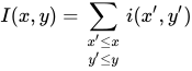
La tabla de áreas sumadas se puede calcular de manera eficiente en una sola pasada sobre la imagen, ya que el valor en la tabla de áreas sumadas en ( x , y ) es simplemente: ^{[ 5 ]} $${\displaystyle I(x,y)=i(x,y)+I(x,y-1)+I(x-1,y)-I(x-1,y-1)}$$(Tenga en cuenta que la matriz resultante se calcula desde la esquina superior izquierda).

Once the summed-area table has been computed, evaluating the sum of intensities over any rectangular area requires exactly four array references regardless of the area size. That is, the notation in the figure at right, having A = (x₀, y₀), B = (x₁, y₀), C = (x₀, y₁) and D = (x₁, y₁), the sum of i(x,y) over the rectangle spanned by A, B, C, and D is: $${\displaystyle \sum _{\begin{smallmatrix}x_{0}<x\leq x_{1}\\y_{0}<y\leq y_{1}\end{smallmatrix}}i(x,y)=I(D)+I(A)-I(B)-I(C)}$$

This method is naturally extended to continuous domains.^[2]

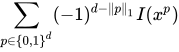
The method can be also extended to high-dimensional images.^[6] If the corners of the rectangle are ${\displaystyle x^{p}}$ with ${\displaystyle p}$ in ${\displaystyle \{0,1\}^{d}}$, then the sum of image values contained in the rectangle are computed with the formula $${\displaystyle \sum _{p\in \{0,1\}^{d}}(-1)^{d-\|p\|_{1}}I(x^{p})}$$ where ${\displaystyle I(x)}$ is the integral image at ${\displaystyle x}$ and ${\displaystyle d}$ the image dimension. The notation ${\displaystyle x^{p}}$ correspond in the example to ${\displaystyle d=2}$, ${\displaystyle A=x^{(0,0)}}$, ${\displaystyle B=x^{(1,0)}}$, ${\displaystyle C=x^{(1,1)}}$ and ${\displaystyle D=x^{(0,1)}}$. In neuroimaging, for example, the images have dimension ${\displaystyle d=3}$ or ${\displaystyle d=4}$, when using voxels or voxels with a time-stamp.

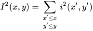
This method has been extended to high-order integral image as in the work of Phan et al.^[7] who provided two, three, or four integral images for quickly and efficiently calculating the standard deviation (variance), skewness, and kurtosis of local block in the image. This is detailed below:

To compute variance or standard deviation of a block, we need two integral images: $${\displaystyle I(x,y)=\sum _{\begin{smallmatrix}x'\leq x\\y'\leq y\end{smallmatrix}}i(x',y')}$$$${\displaystyle I^{2}(x,y)=\sum _{\begin{smallmatrix}x'\leq x\\y'\leq y\end{smallmatrix}}i^{2}(x',y')}$$ The variance is given by: $${\displaystyle \operatorname {Var} (X)={\frac {1}{n}}\sum _{i=1}^{n}(x_{i}-\mu )^{2}.}$$ Let ${\displaystyle S_{1}}$ and ${\displaystyle S_{2}}$ denote the summations of block ${\displaystyle ABCD}$ of ${\displaystyle I}$ and ${\displaystyle I^{2}}$, respectively. ${\displaystyle S_{1}}$ and ${\displaystyle S_{2}}$ are computed quickly by integral image. 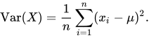Now, we manipulate the variance equation as: $${\displaystyle {\begin{aligned}\operatorname {Var} (X)&={\frac {1}{n}}\sum _{i=1}^{n}\left(x_{i}^{2}-2\mu x_{i}+\mu ^{2}\right)\\[1ex]&={\frac {1}{n}}\left[\sum _{i=1}^{n}x_{i}^{2}-2\sum _{i=1}^{n}\mu x_{i}+\sum _{i=1}^{n}\mu ^{2}\right]\\[1ex]&={\frac {1}{n}}\left[\sum _{i=1}^{n}x_{i}^{2}-2\sum _{i=1}^{n}\mu x_{i}+n\mu ^{2}\right]\\[1ex]&={\frac {1}{n}}\left[\sum _{i=1}^{n}x_{i}^{2}-2\mu \sum _{i=1}^{n}x_{i}+n\mu ^{2}\right]\\[1ex]&={\frac {1}{n}}\left[S_{2}-2{\frac {S_{1}}{n}}S_{1}+n\left({\frac {S_{1}}{n}}\right)^{2}\right]\\[1ex]&={\frac {1}{n}}\left[S_{2}-{\frac {S_{1}^{2}}{n}}\right]\end{aligned}}}$$ Where ${\displaystyle \mu =S_{1}/n}$ and ${\textstyle S_{2}=\sum _{i=1}^{n}x_{i}^{2}}$.

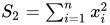
Similar to the estimation of the mean (${\displaystyle \mu }$) and variance (${\displaystyle \operatorname {Var} }$), which requires the integral images of the first and second power of the image respectively (i.e. ${\displaystyle I,I^{2}}$); manipulations similar to the ones mentioned above can be made to the third and fourth powers of the images (i.e. ${\displaystyle I^{3}(x,y),I^{4}(x,y)}$.) for obtaining the skewness and kurtosis.^[7] But one important implementation detail that must be kept in mind for the above methods, as mentioned by F Shafait et al.^[8] is that of integer overflow occurring for the higher order integral images in case 32-bit integers are used.

Es posible que el tipo de datos para las sumas deba ser diferente y de mayor tamaño que el tipo de datos utilizado para los valores originales, para poder acomodar la suma máxima esperada sin desbordamiento . Para datos de punto flotante, el error se puede reducir mediante la suma compensada .

• Suma de prefijo

• Implementación de tablas sumadas en la detección de objetos