Articulo de referencia

Ondícula spline

Animación que muestra las ondículas B-spline cardinales con soporte compacto de órdenes 1, 2, 3, 4 y 5. En la teoría matemática de las ondículas , una ondícula spline es una ond...

Animación que muestra las ondículas B-spline cardinales con soporte compacto de órdenes 1, 2, 3, 4 y 5.

En la teoría matemática de las ondículas , una ondícula spline es una ondícula construida utilizando una función spline . [ 1 ] Existen diferentes tipos de ondículas spline. Las ondículas spline interpoladoras introducidas por CK Chui y JZ Wang se basan en una fórmula de interpolación spline específica. [ 2 ] Aunque estas ondículas son ortogonales , no tienen soportes compactos . Existe una clase particular de ondículas, únicas en cierto sentido, construidas utilizando B-splines y con soportes compactos. Si bien estas ondículas no son ortogonales, poseen propiedades especiales que las han hecho muy populares. [ 3 ] El término ondícula spline se utiliza a veces para referirse a las ondículas de esta clase. Estas ondículas especiales también se denominan ondículas B-spline y ondículas B-spline cardinales . [ 4 ] Las ondículas de Battle-Lemarie también son ondículas construidas utilizando funciones spline. [ 5 ]

Splines B cardinales

Sea n un entero fijo no negativo . Sea C n el conjunto de todas las funciones de valor real definidas sobre el conjunto de números reales tales que cada función en el conjunto, así como sus primeras n derivadas, son continuas en todas partes. Una secuencia bi-infinita . . . x −2 , x −1 , x 0 , x 1 , x 2 , . . . tal que x r < x r +1 para todo r y tal que x r se aproxima a ±∞ cuando r se aproxima a ±∞ se dice que define un conjunto de nudos. Una spline de orden n con un conjunto de nudos { x r } es una función S ( x ) en C n tal que, para cada r , la restricción de S ( x ) al intervalo [ x r , x r +1 ) coincide con un polinomio con coeficientes reales de grado como máximo n en x .

Si la separación x r +1 - x r , donde r es cualquier entero, entre los nodos sucesivos del conjunto de nodos es constante, la spline se denomina spline cardinal . El conjunto de enteros Z = {..., -2, -1, 0, 1, 2, ...} es una elección estándar para el conjunto de nodos de una spline cardinal. Salvo que se especifique lo contrario, generalmente se asume que el conjunto de nodos es el conjunto de enteros.

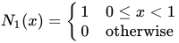
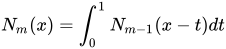
Una B-spline cardinal es un tipo especial de spline cardinal. Para cualquier entero positivo m, la B-spline cardinal de orden m , denotada por N m ( x ), se define recursivamente de la siguiente manera.

norte1(incógnita)={10incógnita<10de lo contrario{\displaystyle N_{1}(x)={\begin{cases}1&0\leq x<1\\0&{\text{en otro caso}}\end{cases}}}
nortemetro(incógnita)=01nortemetro1(incógnitat)dt{\displaystyle N_{m}(x)=\int _{0}^{1}N_{m-1}(xt)dt}, parametro>1{\displaystyle m>1}.

Más adelante en este artículo se presentan expresiones concretas para las B-splines cardinales de todos los órdenes hasta 5 y sus gráficas.

Propiedades de las B-splines cardinales

Propiedades elementales

  1. El apoyo denortemetro(incógnita){\displaystyle N_{m}(x)}es el intervalo cerrado[0,metro]{\displaystyle [0,m]}.
  2. La funciónnortemetro(incógnita){\displaystyle N_{m}(x)}es no negativo, es decir,nortemetro(incógnita)>0{\displaystyle N_{m}(x)>0}para0<incógnita<metro{\displaystyle 0<x<m}.
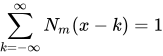
  3. k=nortemetro(incógnitak)=1{\displaystyle \sum _{k=-\infty }^{\infty }N_{m}(xk)=1}a pesar deincógnita{\displaystyle x}.
  4. Las B-splines cardinales de órdenes m y m-1 están relacionadas por la identidad:nortemetro(incógnita)=incógnitametronortemetro1(incógnita)+metro+1incógnitametronortemetro1(incógnita1){\displaystyle N_{m}(x)={\frac {x}{m}}N_{m-1}(x)+{\frac {m+1-x}{m}}N_{m-1}(x-1)}.
  5. La funciónnortemetro(incógnita){\displaystyle N_{m}(x)}es simétrico respecto aincógnita=metro2{\displaystyle x={\frac {m}{2}}}, eso es,nortemetro(metro2incógnita)=nortemetro(metro2+incógnita){\displaystyle N_{m}\left({\frac {m}{2}}-x\right)=N_{m}\left({\frac {m}{2}}+x\right)}.
  6. El derivado denortemetro(incógnita){\displaystyle N_{m}(x)}es dado pornortemetro(incógnita)=nortemetro1(incógnita)nortemetro1(incógnita1){\displaystyle N_{m}^{\prime }(x)=N_{m-1}(x)-N_{m-1}(x-1)}.
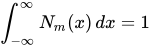
  7. nortemetro(incógnita)dincógnita=1{\displaystyle \int _{-\infty }^{\infty }N_{m}(x)\,dx=1}

Relación de dos escalas

The cardinal B-spline of order m satisfies the following two-scale relation:

Nm(x)=k=0m2m+1(mk)Nm(2xk){\displaystyle N_{m}(x)=\sum _{k=0}^{m}2^{-m+1}{m \choose k}N_{m}(2x-k)}.

Riesz property

The cardinal B-spline of order m satisfies the following property, known as the Riesz property: There exists two positive real numbers A{\displaystyle A} and B{\displaystyle B} such that for any square summable two-sided sequence {ck}k={\displaystyle \{c_{k}\}_{k=-\infty }^{\infty }} and for any x,

A{ck}2k=ckNm(xk)2B{ck}2{\displaystyle A\left\Vert \{c_{k}\}\right\Vert ^{2}\leq \left\Vert \sum _{k=-\infty }^{\infty }c_{k}N_{m}(x-k)\right\Vert ^{2}\leq B\left\Vert \{c_{k}\}\right\Vert ^{2}}

where {\displaystyle \Vert \cdot \Vert } is the norm in the ℓ2-space.

Cardinal B-splines of small orders

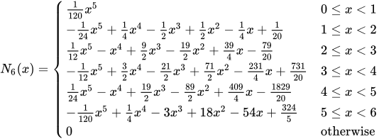
The cardinal B-splines are defined recursively starting from the B-spline of order 1, namely N1(x){\displaystyle N_{1}(x)}, which takes the value 1 in the interval [0, 1) and 0 elsewhere. Computer algebra systems may have to be employed to obtain concrete expressions for higher order cardinal B-splines. The concrete expressions for cardinal B-splines of all orders up to 6 are given below. The graphs of cardinal B-splines of orders up to 4 are also exhibited. In the images, the graphs of the terms contributing to the corresponding two-scale relations are also shown. The two dots in each image indicate the extremities of the interval supporting the B-spline.

Constant B-spline

The B-spline of order 1, namely N1(x){\displaystyle N_{1}(x)}, is the constant B-spline. It is defined by

N1(x)={10x<10otherwise{\displaystyle N_{1}(x)={\begin{cases}1&0\leq x<1\\0&{\text{otherwise}}\end{cases}}}

The two-scale relation for this B-spline is

N1(x)=N1(2x)+N1(2x1){\displaystyle N_{1}(x)=N_{1}(2x)+N_{1}(2x-1)}

Linear B-spline

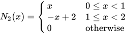
The B-spline of order 2, namely N2(x){\displaystyle N_{2}(x)}, is the linear B-spline. It is given by

N2(x)={x0x<1x+21x<20otherwise{\displaystyle N_{2}(x)={\begin{cases}x&0\leq x<1\\-x+2&1\leq x<2\\0&{\text{otherwise}}\end{cases}}}

The two-scale relation for this wavelet is

N2(x)=12N2(2x)+N2(2x1)+12N2(2x2){\displaystyle N_{2}(x)={\frac {1}{2}}N_{2}(2x)+N_{2}(2x-1)+{\frac {1}{2}}N_{2}(2x-2)}

Quadratic B-spline

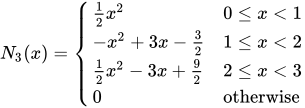
The B-spline of order 3, namely N3(x){\displaystyle N_{3}(x)}, is the quadratic B-spline. It is given by

N3(x)={12x20x<1x2+3x321x<212x23x+922x<30otherwise{\displaystyle N_{3}(x)={\begin{cases}{\frac {1}{2}}x^{2}&0\leq x<1\\-x^{2}+3x-{\frac {3}{2}}&1\leq x<2\\{\frac {1}{2}}x^{2}-3x+{\frac {9}{2}}&2\leq x<3\\0&{\text{otherwise}}\end{cases}}}

The two-scale relation for this wavelet is

N3(x)=14N3(2x)+34N3(2x1)+34N3(2x2)+14N3(2x3){\displaystyle N_{3}(x)={\frac {1}{4}}N_{3}(2x)+{\frac {3}{4}}N_{3}(2x-1)+{\frac {3}{4}}N_{3}(2x-2)+{\frac {1}{4}}N_{3}(2x-3)}

Cubic B-spline

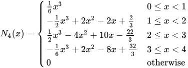
The cubic B-spline is the cardinal B-spline of order 4, denoted by N4(x){\displaystyle N_{4}(x)}. It is given by the following expressions:

N4(x)={16x30x<112x3+2x22x+231x<212x34x2+10x2232x<316x3+2x28x+3233x<40otherwise{\displaystyle N_{4}(x)={\begin{cases}{\frac {1}{6}}x^{3}&0\leq x<1\\-{\frac {1}{2}}x^{3}+2x^{2}-2x+{\frac {2}{3}}&1\leq x<2\\{\frac {1}{2}}x^{3}-4x^{2}+10x-{\frac {22}{3}}&2\leq x<3\\-{\frac {1}{6}}x^{3}+2x^{2}-8x+{\frac {32}{3}}&3\leq x<4\\0&{\text{otherwise}}\end{cases}}}

The two-scale relation for the cubic B-spline is

N4(x)=18N4(2x)+12N4(2x1)+34N4(2x2)+12N4(2x3)+18N4(2x4){\displaystyle N_{4}(x)={\frac {1}{8}}N_{4}(2x)+{\frac {1}{2}}N_{4}(2x-1)+{\frac {3}{4}}N_{4}(2x-2)+{\frac {1}{2}}N_{4}(2x-3)+{\frac {1}{8}}N_{4}(2x-4)}

Bi-quadratic B-spline

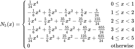
The bi-quadratic B-spline is the cardinal B-spline of order 5 denoted by N5(x){\displaystyle N_{5}(x)}. It is given by

N5(x)={124x40x<116x4+56x354x2+56x5241x<214x452x3+354x2252x+155242x<316x4+52x3554x2+652x655243x<4124x456x3+254x21256x+625244x<50otherwise{\displaystyle N_{5}(x)={\begin{cases}{\frac {1}{24}}x^{4}&0\leq x<1\\-{\frac {1}{6}}x^{4}+{\frac {5}{6}}x^{3}-{\frac {5}{4}}x^{2}+{\frac {5}{6}}x-{\frac {5}{24}}&1\leq x<2\\{\frac {1}{4}}x^{4}-{\frac {5}{2}}x^{3}+{\frac {35}{4}}x^{2}-{\frac {25}{2}}x+{\frac {155}{24}}&2\leq x<3\\-{\frac {1}{6}}x^{4}+{\frac {5}{2}}x^{3}-{\frac {55}{4}}x^{2}+{\frac {65}{2}}x-{\frac {655}{24}}&3\leq x<4\\{\frac {1}{24}}x^{4}-{\frac {5}{6}}x^{3}+{\frac {25}{4}}x^{2}-{\frac {125}{6}}x+{\frac {625}{24}}&4\leq x<5\\0&{\text{otherwise}}\end{cases}}}

The two-scale relation is

N5(x)=116N5(2x)+516N5(2x1)+1016N5(2x2)+1016N5(2x3)+516N5(2x4)+116N5(2x5){\displaystyle N_{5}(x)={\frac {1}{16}}N_{5}(2x)+{\frac {5}{16}}N_{5}(2x-1)+{\frac {10}{16}}N_{5}(2x-2)+{\frac {10}{16}}N_{5}(2x-3)+{\frac {5}{16}}N_{5}(2x-4)+{\frac {1}{16}}N_{5}(2x-5)}

Quintic B-spline

The quintic B-spline is the cardinal B-spline of order 6 denoted by N6(x){\displaystyle N_{6}(x)}. It is given by

N6(x)={1120x50x<1124x5+14x412x3+12x214x+1201x<2112x5x4+92x3192x2+394x79202x<3112x5+32x4212x3+712x22314x+731203x<4124x5x4+192x3892x2+4094x1829204x<51120x5+14x43x3+18x254x+32455x<60otherwise{\displaystyle N_{6}(x)={\begin{cases}{\frac {1}{120}}x^{5}&0\leq x<1\\-{\frac {1}{24}}x^{5}+{\frac {1}{4}}x^{4}-{\frac {1}{2}}x^{3}+{\frac {1}{2}}x^{2}-{\frac {1}{4}}x+{\frac {1}{20}}&1\leq x<2\\{\frac {1}{12}}x^{5}-x^{4}+{\frac {9}{2}}x^{3}-{\frac {19}{2}}x^{2}+{\frac {39}{4}}x-{\frac {79}{20}}&2\leq x<3\\-{\frac {1}{12}}x^{5}+{\frac {3}{2}}x^{4}-{\frac {21}{2}}x^{3}+{\frac {71}{2}}x^{2}-{\frac {231}{4}}x+{\frac {731}{20}}&3\leq x<4\\{\frac {1}{24}}x^{5}-x^{4}+{\frac {19}{2}}x^{3}-{\frac {89}{2}}x^{2}+{\frac {409}{4}}x-{\frac {1829}{20}}&4\leq x<5\\-{\frac {1}{120}}x^{5}+{\frac {1}{4}}x^{4}-3x^{3}+18x^{2}-54x+{\frac {324}{5}}&5\leq x<6\\0&{\text{otherwise}}\end{cases}}}

Multi-resolution analysis generated by cardinal B-splines

The cardinal B-spline Nm(x){\displaystyle N_{m}(x)} of order m generates a multi-resolution analysis. In fact, from the elementary properties of these functions enunciated above, it follows that the function Nm(x){\displaystyle N_{m}(x)} is square integrable and is an element of the space L2(R){\displaystyle L^{2}(R)} of square integrable functions. To set up the multi-resolution analysis the following notations used.

  • For any integers k,j{\displaystyle k,j}, define the function Nm,kj(x)=Nm(2kxj){\displaystyle N_{m,kj}(x)=N_{m}(2^{k}x-j)}.
  • For each integer k{\displaystyle k}, define the subspace Vk{\displaystyle V_{k}} of L2(R){\displaystyle L^{2}(R)} as the closure of the linear span of the set {Nm,kj(x):j=,2,1,0,1,2,}{\displaystyle \{N_{m,kj}(x):j=\cdots ,-2,-1,0,1,2,\cdots \}}.

That these define a multi-resolution analysis follows from the following:

  1. The spaces Vk{\displaystyle V_{k}} satisfy the property: V2V1V0V1V2{\displaystyle \cdots \subset V_{-2}\subset V_{-1}\subset V_{0}\subset V_{1}\subset V_{2}\subset \cdots }.
  2. The closure in L2(R){\displaystyle L^{2}(R)} of the union of all the subspaces Vk{\displaystyle V_{k}} is the whole space L2(R){\displaystyle L^{2}(R)}.
  3. The intersection of all the subspaces Vk{\displaystyle V_{k}} is the singleton set containing only the zero function.
  4. For each integer k{\displaystyle k} the set {Nm,kj(x):j=,2,1,0,1,2,}{\displaystyle \{N_{m,kj}(x):j=\cdots ,-2,-1,0,1,2,\cdots \}} is an unconditional basis for Vk{\displaystyle V_{k}}. (A sequence {xn} in a Banach space X is an unconditional basis for the space X if every permutation of the sequence {xn} is also a basis for the same space X.[6])

Wavelets from cardinal B-splines

Let m be a fixed positive integer and Nm(x){\displaystyle N_{m}(x)} be the cardinal B-spline of order m. A function ψm(x){\displaystyle \psi _{m}(x)} in L2(R){\displaystyle L^{2}(R)} is a basic wavelet relative to the cardinal B-spline function Nm(x){\displaystyle N_{m}(x)} if the closure in L2(R){\displaystyle L^{2}(R)} of the linear span of the set {ψm(xj):j=,2,1,0,1,2,}{\displaystyle \{\psi _{m}(x-j):j=\cdots ,-2,-1,0,1,2,\cdots \}} (this closure is denoted by W0{\displaystyle W_{0}}) is the orthogonal complement of V0{\displaystyle V_{0}} in V1{\displaystyle V_{1}}. The subscript m in ψm(x){\displaystyle \psi _{m}(x)} is used to indicate that ψm(x){\displaystyle \psi _{m}(x)} is a basic wavelet relative the cardinal B-spline of order m. There is no unique basic wavelet ψm(x){\displaystyle \psi _{m}(x)} relative to the cardinal B-spline Nm(x){\displaystyle N_{m}(x)}. Some of these are discussed in the following sections.

Wavelets relative to cardinal B-splines using fundamental interpolatory splines

Fundamental interpolatory spline

Definitions

Let m be a fixed positive integer and let Nm(x){\displaystyle N_{m}(x)} be the cardinal B-spline of order m. Given a sequence {fj:j=,2,1,0,1,2,}{\displaystyle \{f_{j}:j=\cdots ,-2,-1,0,1,2,\cdots \}} of real numbers, the problem of finding a sequence {cm,k:k=,2,1,0,1,2,}{\displaystyle \{c_{m,k}:k=\cdots ,-2,-1,0,1,2,\cdots \}} of real numbers such that

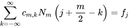
k=cm,kNm(j+m2k)=fj{\displaystyle \sum _{k=-\infty }^{\infty }c_{m,k}N_{m}\left(j+{\frac {m}{2}}-k\right)=f_{j}} for all j{\displaystyle j},

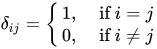
is known as the cardinal spline interpolation problem. The special case of this problem where the sequence {fj}{\displaystyle \{f_{j}\}} is the sequence δ0j{\displaystyle \delta _{0j}}, where δij{\displaystyle \delta _{ij}} is the Kronecker delta function δij{\displaystyle \delta _{ij}} defined by

δij={1, if i=j0, if ij{\displaystyle \delta _{ij}={\begin{cases}1,&{\text{ if }}i=j\\0,&{\text{ if }}i\neq j\end{cases}}},

is the fundamental cardinal spline interpolation problem. The solution of the problem yields the fundamental cardinal interpolatory spline of order m. This spline is denoted by Lm(x){\displaystyle L_{m}(x)} and is given by

Lm(x)=k=cm,kNm(x+m2k){\displaystyle L_{m}(x)=\sum _{k=-\infty }^{\infty }c_{m,k}N_{m}\left(x+{\frac {m}{2}}-k\right)}

where the sequence {cm,k}{\displaystyle \{c_{m,k}\}} is now the solution of the following system of equations:

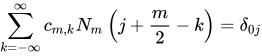
k=cm,kNm(j+m2k)=δ0j{\displaystyle \sum _{k=-\infty }^{\infty }c_{m,k}N_{m}\left(j+{\frac {m}{2}}-k\right)=\delta _{0j}}

Procedure to find the fundamental cardinal interpolatory spline

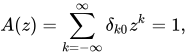
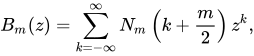
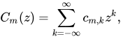
The fundamental cardinal interpolatory spline Lm(x){\displaystyle L_{m}(x)} can be determined using Z-transforms. Using the following notations

A(z)=k=δk0zk=1,{\displaystyle A(z)=\sum _{k=-\infty }^{\infty }\delta _{k0}z^{k}=1,}
Bm(z)=k=Nm(k+m2)zk,{\displaystyle B_{m}(z)=\sum _{k=-\infty }^{\infty }N_{m}\left(k+{\frac {m}{2}}\right)z^{k},}
Cm(z)=k=cm,kzk,{\displaystyle C_{m}(z)=\sum _{k=-\infty }^{\infty }c_{m,k}z^{k},}

it can be seen from the equations defining the sequence cm,k{\displaystyle c_{m,k}} that

Bm(z)Cm(z)=A(z){\displaystyle B_{m}(z)C_{m}(z)=A(z)}

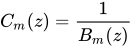
from which we get

Cm(z)=1Bm(z){\displaystyle C_{m}(z)={\frac {1}{B_{m}(z)}}}.

This can be used to obtain concrete expressions for cm,k{\displaystyle c_{m,k}}.

Example

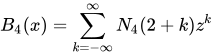
As a concrete example, the case L4(x){\displaystyle L_{4}(x)} may be investigated. The definition of Bm(z){\displaystyle B_{m}(z)} implies that

B4(x)=k=N4(2+k)zk{\displaystyle B_{4}(x)=\sum _{k=-\infty }^{\infty }N_{4}(2+k)z^{k}}

The only nonzero values of N4(k+2){\displaystyle N_{4}(k+2)} are given by k=1,0,1{\displaystyle k=-1,0,1} and the corresponding values are

N4(1)=16,N4(2)=46,N4(3)=16.{\displaystyle N_{4}(1)={\frac {1}{6}},N_{4}(2)={\frac {4}{6}},N_{4}(3)={\frac {1}{6}}.}

Thus B4(z){\displaystyle B_{4}(z)} reduces to

B4(z)=16z1+46z0+16z1=1+4z+z26z{\displaystyle B_{4}(z)={\frac {1}{6}}z^{-1}+{\frac {4}{6}}z^{0}+{\frac {1}{6}}z^{1}={\frac {1+4z+z^{2}}{6z}}}

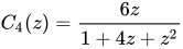
This yields the following expression for C4(z){\displaystyle C_{4}(z)}.

C4(z)=6z1+4z+z2{\displaystyle C_{4}(z)={\frac {6z}{1+4z+z^{2}}}}

Splitting this expression into partial fractions and expanding each term in powers of z in an annular region the values of c4,k{\displaystyle c_{4,k}} can be computed. These values are then substituted in the expression for L4(x){\displaystyle L_{4}(x)} to yield

L4(x)=k=(1)k3(23)|k|N4(x+2k){\displaystyle L_{4}(x)=\sum _{k=-\infty }^{\infty }(-1)^{k}{\sqrt {3}}(2-{\sqrt {3}})^{|k|}N_{4}(x+2-k)}

Wavelet using fundamental interpolatory spline

For a positive integer m, the function ψm(x){\displaystyle \psi _{m}(x)} defined by

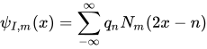
ψI,m(x)=dmdxmL2m(2x1){\displaystyle \psi _{I,m}(x)={\frac {d^{m}}{dx^{m}}}L_{2m}(2x-1)}

is a basic wavelet relative to the cardinal B-spline of order Nm(x){\displaystyle N_{m}(x)}. The subscript I in ψI,m{\displaystyle \psi _{I,m}} is used to indicate that it is based in the interpolatory spline formula. This basic wavelet is not compactly supported.

Example

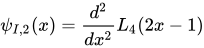
The wavelet of order 2 using interpolatory spline is given by

ψI,2(x)=d2dx2L4(2x1){\displaystyle \psi _{I,2}(x)={\frac {d^{2}}{dx^{2}}}L_{4}(2x-1)}

The expression for L4(x){\displaystyle L_{4}(x)} now yields the following formula:

ψI,2(x)=d2dx2k=(1)k3(23)|k|N4(2x+1k){\displaystyle \psi _{I,2}(x)={\frac {d^{2}}{dx^{2}}}\sum _{k=-\infty }^{\infty }(-1)^{k}{\sqrt {3}}(2-{\sqrt {3}})^{|k|}N_{4}(2x+1-k)}

Now, using the expression for the derivative of Nm(x){\displaystyle N_{m}(x)} in terms of Nm1(x){\displaystyle N_{m-1}(x)} the function ψ2(x){\displaystyle \psi _{2}(x)} can be put in the following form:

ψI,2(x)=k=(1)k43(23)|k|((N2(2x+k1)2N2(2x+k2)+N2(2x+k3)){\displaystyle \psi _{I,2}(x)=\sum _{k=-\infty }^{\infty }(-1)^{k}4{\sqrt {3}}(2-{\sqrt {3}})^{|k|}{\Big (}(N_{2}(2x+k-1)-2N_{2}(2x+k-2)+N_{2}(2x+k-3){\Big )}}

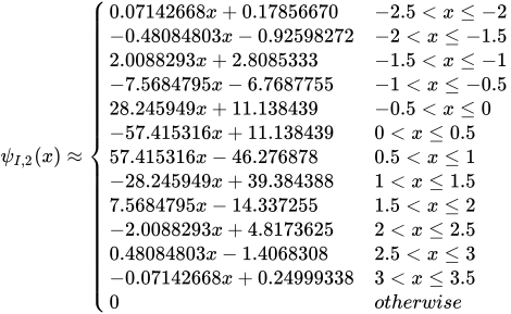
The following piecewise linear function is the approximation to ψ2(x){\displaystyle \psi _{2}(x)} obtained by taking the sum of the terms corresponding to k=3,,3{\displaystyle k=-3,\ldots ,3} in the infinite series expression for ψ2(x){\displaystyle \psi _{2}(x)}.

ψI,2(x){0.07142668x+0.178566702.5<x20.48084803x0.925982722<x1.52.0088293x+2.80853331.5<x17.5684795x6.76877551<x0.528.245949x+11.1384390.5<x057.415316x+11.1384390<x0.557.415316x46.2768780.5<x128.245949x+39.3843881<x1.57.5684795x14.3372551.5<x22.0088293x+4.81736252<x2.50.48084803x1.40683082.5<x30.07142668x+0.249993383<x3.50otherwise{\displaystyle \psi _{I,2}(x)\approx {\begin{cases}0.07142668x+0.17856670&-2.5<x\leq -2\\-0.48084803x-0.92598272&-2<x\leq -1.5\\2.0088293x+2.8085333&-1.5<x\leq -1\\-7.5684795x-6.7687755&-1<x\leq -0.5\\28.245949x+11.138439&-0.5<x\leq 0\\-57.415316x+11.138439&0<x\leq 0.5\\57.415316x-46.276878&0.5<x\leq 1\\-28.245949x+39.384388&1<x\leq 1.5\\7.5684795x-14.337255&1.5<x\leq 2\\-2.0088293x+4.8173625&2<x\leq 2.5\\0.48084803x-1.4068308&2.5<x\leq 3\\-0.07142668x+0.24999338&3<x\leq 3.5\\0&{otherwise}\end{cases}}}

Two-scale relation

The two-scale relation for the wavelet function ψm(x){\displaystyle \psi _{m}(x)} is given by

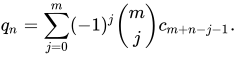
ψI,m(x)=qnNm(2xn){\displaystyle \psi _{I,m}(x)=\sum _{-\infty }^{\infty }q_{n}N_{m}(2x-n)} where qn=j=0m(1)j(mj)cm+nj1.{\displaystyle q_{n}=\sum _{j=0}^{m}(-1)^{j}{m \choose j}c_{m+n-j-1}.}

Compactly supported B-spline wavelets

The spline wavelets generated using the interpolatory wavelets are not compactly supported. Compactly supported B-spline wavelets were discovered by Charles K. Chui and Jian-zhong Wang and published in 1991.[3][7] The compactly supported B-spline wavelet relative to the cardinal B-spline Nm(x){\displaystyle N_{m}(x)} of order m discovered by Chui and Wang and denoted by ψC,m(x){\displaystyle \psi _{C,m}(x)}, has as its support the interval [0,2m1]{\displaystyle [0,2m-1]}. These wavelets are essentially unique in a certain sense explained below.

Definition

The compactly supported B-spline wavelet of order m is given by

ψC,m(x)=12m1j=02m2(1)jN2m(j+1)dmdxmN2m(2xj){\displaystyle \psi _{C,m}(x)={\frac {1}{2^{m-1}}}\sum _{j=0}^{2m-2}(-1)^{j}N_{2m}(j+1){\frac {d^{m}}{dx^{m}}}N_{2m}(2x-j)}

This is an m-th order spline. As a special case, the compactly supported B-spline wavelet of order 1 is

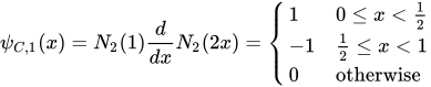
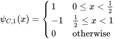
ψC,1(x)=N2(1)ddxN2(2x)={10x<12112x<10otherwise{\displaystyle \psi _{C,1}(x)=N_{2}(1){\frac {d}{dx}}N_{2}(2x)={\begin{cases}1&0\leq x<{\frac {1}{2}}\\-1&{\frac {1}{2}}\leq x<1\\0&{\text{otherwise}}\end{cases}}}

which is the well-known Haar wavelet.

Properties

  1. The support of ψC,m(x){\displaystyle \psi _{C,m}(x)} is the closed interval [0,2m1]{\displaystyle [0,2m-1]}.
  2. The wavelet ψC,m(x){\displaystyle \psi _{C,m}(x)} is the unique wavelet with minimum support in the following sense: If η(x)W0{\displaystyle \eta (x)\in W_{0}} generates W0{\displaystyle W_{0}} and has support not exceeding 2m1{\displaystyle 2m-1} in length then η(x)=c0ψC,m(xn0){\displaystyle \eta (x)=c_{0}\psi _{C,m}(x-n_{0})} for some nonzero constant c0{\displaystyle c_{0}} and for some integer n0{\displaystyle n_{0}}.[8]
  3. ψC,m(x){\displaystyle \psi _{C,m}(x)} is symmetric for even m and antisymmetric for odd m.

Two-scale relation

ψm(x){\displaystyle \psi _{m}(x)} satisfies the two-scale relation:

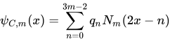
ψC,m(x)=n=03m2qnNm(2xn){\displaystyle \psi _{C,m}(x)=\sum _{n=0}^{3m-2}q_{n}N_{m}(2x-n)} where qn=(1)n2m1j=0m(mj)N2m(nj+1){\displaystyle q_{n}={\frac {(-1)^{n}}{2^{m-1}}}\sum _{j=0}^{m}{m \choose j}N_{2m}(n-j+1)}.

Decomposition relation

The decomposition relation for the compactly supported B-spline wavelet has the following form:

Nm(2xl)=k=[am,l2kNm(xk)+bm,l2kψC,m(xk)]{\displaystyle N_{m}(2x-l)=\sum _{k=-\infty }^{\infty }\left[a_{m,l-2k}N_{m}(x-k)+b_{m,l-2k}\psi _{C,m}(x-k)\right]}

where the coefficients am,j{\displaystyle a_{m,j}} and bm,j{\displaystyle b_{m,j}} are given by

am,j=(1)j2l=qj+2m2l+1c2m,l,{\displaystyle a_{m,j}=-{\frac {(-1)^{j}}{2}}\sum _{l=-\infty }^{\infty }q_{-j+2m-2l+1}c_{2m,l},}
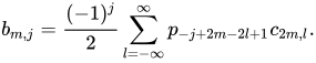
bm,j=(1)j2l=pj+2m2l+1c2m,l.{\displaystyle b_{m,j}={\frac {(-1)^{j}}{2}}\sum _{l=-\infty }^{\infty }p_{-j+2m-2l+1}c_{2m,l}.}

Here the sequence c2m,l{\displaystyle c_{2m,l}} is the sequence of coefficients in the fundamental interpolatoty cardinal spline wavelet of order m.

Compactly supported B-spline wavelets of small orders

Compactly supported B-spline wavelet of order 1

The two-scale relation for the compactly supported B-spline wavelet of order 1 is

ψC,1(x)=N1(2x)N1(2x1){\displaystyle \psi _{C,1}(x)=N_{1}(2x)-N_{1}(2x-1)}

The closed form expression for compactly supported B-spline wavelet of order 1 is

ψC,1(x)={10x<12112x<10otherwise{\displaystyle \psi _{C,1}(x)={\begin{cases}1&0\leq x<{\frac {1}{2}}\\-1&{\frac {1}{2}}\leq x<1\\0&{\text{otherwise}}\end{cases}}}

Compactly supported B-spline wavelet of order 2

The two-scale relation for the compactly supported B-spline wavelet of order 2 is

ψC,2(x)=112(N2(2x)6N2(2x1)+10N2(2x2)6N2(2x3)+N2(2x4)){\displaystyle \psi _{C,2}(x)={\frac {1}{12}}\left(N_{2}(2x)-6N_{2}(2x-1)+10N_{2}(2x-2)-6N_{2}(2x-3)+N_{2}(2x-4)\right)}

The closed form expression for compactly supported B-spline wavelet of order 2 is

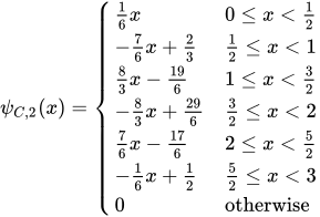
ψC,2(x)={16x0x<1276x+2312x<183x1961x<3283x+29632x<276x1762x<5216x+1252x<30otherwise{\displaystyle \psi _{C,2}(x)={\begin{cases}{\frac {1}{6}}x&0\leq x<{\frac {1}{2}}\\-{\frac {7}{6}}x+{\frac {2}{3}}&{\frac {1}{2}}\leq x<1\\{\frac {8}{3}}x-{\frac {19}{6}}&1\leq x<{\frac {3}{2}}\\-{\frac {8}{3}}x+{\frac {29}{6}}&{\frac {3}{2}}\leq x<2\\{\frac {7}{6}}x-{\frac {17}{6}}&2\leq x<{\frac {5}{2}}\\-{\frac {1}{6}}x+{\frac {1}{2}}&{\frac {5}{2}}\leq x<3\\0&{\text{otherwise}}\end{cases}}}

Compactly supported B-spline wavelet of order 3

The two-scale relation for the compactly supported B-spline wavelet of order 3 is

ψC,3(x)=1480[(N3(2x)29N3(2x1)+147N3(2x2)303N3(2x3)+{\displaystyle \psi _{C,3}(x)={\frac {1}{480}}{\Big [}(N_{3}(2x)-29N_{3}(2x-1)+147N_{3}(2x-2)-303N_{3}(2x-3)+}
303N3(2x4)147N3(2x5)+29N3(2x6)N3(2x7)]{\displaystyle 303N_{3}(2x-4)-147N_{3}(2x-5)+29N_{3}(2x-6)-N_{3}(2x-7){\Big ]}}

The closed form expression for compactly supported B-spline wavelet of order 3 is

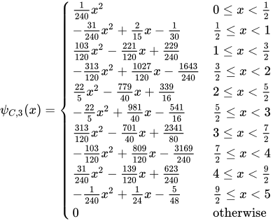
ψC,3(x)={1240x20x<1231240x2+215x13012x<1103120x2221120x+2292401x<32313120x2+1027120x164324032x<2225x277940x+339162x<52225x2+98140x5411652x<3313120x270140x+2341803x<72103120x2+809120x316924072x<431240x2139120x+6232404x<921240x2+124x54892x<50otherwise{\displaystyle \psi _{C,3}(x)={\begin{cases}{\frac {1}{240}}x^{2}&0\leq x<{\frac {1}{2}}\\-{\frac {31}{240}}x^{2}+{\frac {2}{15}}x-{\frac {1}{30}}&{\frac {1}{2}}\leq x<1\\{\frac {103}{120}}x^{2}-{\frac {221}{120}}x+{\frac {229}{240}}&1\leq x<{\frac {3}{2}}\\-{\frac {313}{120}}x^{2}+{\frac {1027}{120}}x-{\frac {1643}{240}}&{\frac {3}{2}}\leq x<2\\{\frac {22}{5}}x^{2}-{\frac {779}{40}}x+{\frac {339}{16}}&2\leq x<{\frac {5}{2}}\\-{\frac {22}{5}}x^{2}+{\frac {981}{40}}x-{\frac {541}{16}}&{\frac {5}{2}}\leq x<3\\{\frac {313}{120}}x^{2}-{\frac {701}{40}}x+{\frac {2341}{80}}&3\leq x<{\frac {7}{2}}\\-{\frac {103}{120}}x^{2}+{\frac {809}{120}}x-{\frac {3169}{240}}&{\frac {7}{2}}\leq x<4\\{\frac {31}{240}}x^{2}-{\frac {139}{120}}x+{\frac {623}{240}}&4\leq x<{\frac {9}{2}}\\-{\frac {1}{240}}x^{2}+{\frac {1}{24}}x-{\frac {5}{48}}&{\frac {9}{2}}\leq x<5\\0&{\text{otherwise}}\end{cases}}}

Compactly supported B-spline wavelet of order 4

The two-scale relation for the compactly supported B-spline wavelet of order 4 is

ψC,4(x)=140320[N4(2x)124N4(2x1)+1677N4(2x2)7904N4(2x3)+18482N4(2x4){\displaystyle \psi _{C,4}(x)={\frac {1}{40320}}{\Big [}N_{4}(2x)-124N_{4}(2x-1)+1677N_{4}(2x-2)-7904N_{4}(2x-3)+18482N_{4}(2x-4)-}
24264N4(2x5)+18482N4(2x6)7904N4(2x7)+1677N4(2x8)124N4(2x9)+N4(2x10)]{\displaystyle 24264N_{4}(2x-5)+18482N_{4}(2x-6)-7904N_{4}(2x-7)+1677N_{4}(2x-8)-124N_{4}(2x-9)+N_{4}(2x-10){\Big ]}}

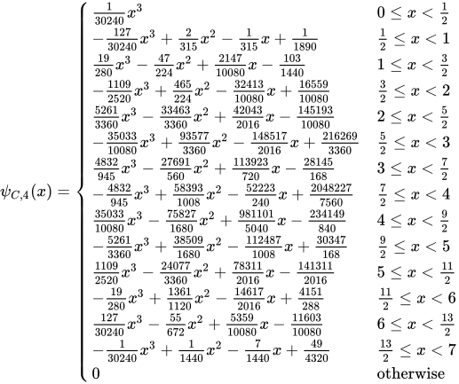
The closed form expression for compactly supported B-spline wavelet of order 4 is

ψC,4(x)={130240x30x<1212730240x3+2315x21315x+1189012x<119280x347224x2+214710080x10314401x<3211092520x3+465224x23241310080x+165591008032x<252613360x3334633360x2+420432016x145193100802x<523503310080x3+935773360x21485172016x+216269336052x<34832945x327691560x2+113923720x281451683x<724832945x3+583931008x252223240x+2048227756072x<43503310080x3758271680x2+9811015040x2341498404x<9252613360x3+385091680x21124871008x+3034716892x<511092520x3240773360x2+783112016x14131120165x<11219280x3+13611120x2146172016x+4151288112x<612730240x355672x2+535910080x11603100806x<132130240x3+11440x271440x+494320132x<70otherwise{\displaystyle \psi _{C,4}(x)={\begin{cases}{\frac {1}{30240}}x^{3}&0\leq x<{\frac {1}{2}}\\-{\frac {127}{30240}}x^{3}+{\frac {2}{315}}x^{2}-{\frac {1}{315}}x+{\frac {1}{1890}}&{\frac {1}{2}}\leq x<1\\{\frac {19}{280}}x^{3}-{\frac {47}{224}}x^{2}+{\frac {2147}{10080}}x-{\frac {103}{1440}}&1\leq x<{\frac {3}{2}}\\-{\frac {1109}{2520}}x^{3}+{\frac {465}{224}}x^{2}-{\frac {32413}{10080}}x+{\frac {16559}{10080}}&{\frac {3}{2}}\leq x<2\\{\frac {5261}{3360}}x^{3}-{\frac {33463}{3360}}x^{2}+{\frac {42043}{2016}}x-{\frac {145193}{10080}}&2\leq x<{\frac {5}{2}}\\-{\frac {35033}{10080}}x^{3}+{\frac {93577}{3360}}x^{2}-{\frac {148517}{2016}}x+{\frac {216269}{3360}}&{\frac {5}{2}}\leq x<3\\{\frac {4832}{945}}x^{3}-{\frac {27691}{560}}x^{2}+{\frac {113923}{720}}x-{\frac {28145}{168}}&3\leq x<{\frac {7}{2}}\\-{\frac {4832}{945}}x^{3}+{\frac {58393}{1008}}x^{2}-{\frac {52223}{240}}x+{\frac {2048227}{7560}}&{\frac {7}{2}}\leq x<4\\{\frac {35033}{10080}}x^{3}-{\frac {75827}{1680}}x^{2}+{\frac {981101}{5040}}x-{\frac {234149}{840}}&4\leq x<{\frac {9}{2}}\\-{\frac {5261}{3360}}x^{3}+{\frac {38509}{1680}}x^{2}-{\frac {112487}{1008}}x+{\frac {30347}{168}}&{\frac {9}{2}}\leq x<5\\{\frac {1109}{2520}}x^{3}-{\frac {24077}{3360}}x^{2}+{\frac {78311}{2016}}x-{\frac {141311}{2016}}&5\leq x<{\frac {11}{2}}\\-{\frac {19}{280}}x^{3}+{\frac {1361}{1120}}x^{2}-{\frac {14617}{2016}}x+{\frac {4151}{288}}&{\frac {11}{2}}\leq x<6\\{\frac {127}{30240}}x^{3}-{\frac {55}{672}}x^{2}+{\frac {5359}{10080}}x-{\frac {11603}{10080}}&6\leq x<{\frac {13}{2}}\\-{\frac {1}{30240}}x^{3}+{\frac {1}{1440}}x^{2}-{\frac {7}{1440}}x+{\frac {49}{4320}}&{\frac {13}{2}}\leq x<7\\0&{\text{otherwise}}\end{cases}}}

Compactly supported B-spline wavelet of order 5

The two-scale relation for the compactly supported B-spline wavelet of order 5 is

ψC,5(x)=15806080[N5(2x)507N5(2x1)+17128N5(2x2)166304N5(2x3)+748465N5(2x4){\displaystyle \psi _{C,5}(x)={\frac {1}{5806080}}{\Big [}N_{5}(2x)-507N_{5}(2x-1)+17128N_{5}(2x-2)-166304N_{5}(2x-3)+748465N_{5}(2x-4)}
1900115N5(2x5)+2973560N5(2x6)2973560N5(2x7)+1900115N5(2x8){\displaystyle -1900115N_{5}(2x-5)+2973560N_{5}(2x-6)-2973560N_{5}(2x-7)+1900115N_{5}(2x-8)}
748465N5(2x9)+166304N5(2x10)17128N5(2x11)+507N5(2x12)N5(2x13)]{\displaystyle -748465N_{5}(2x-9)+166304N_{5}(2x-10)-17128N_{5}(2x-11)+507N_{5}(2x-12)-N_{5}(2x-13){\Big ]}}

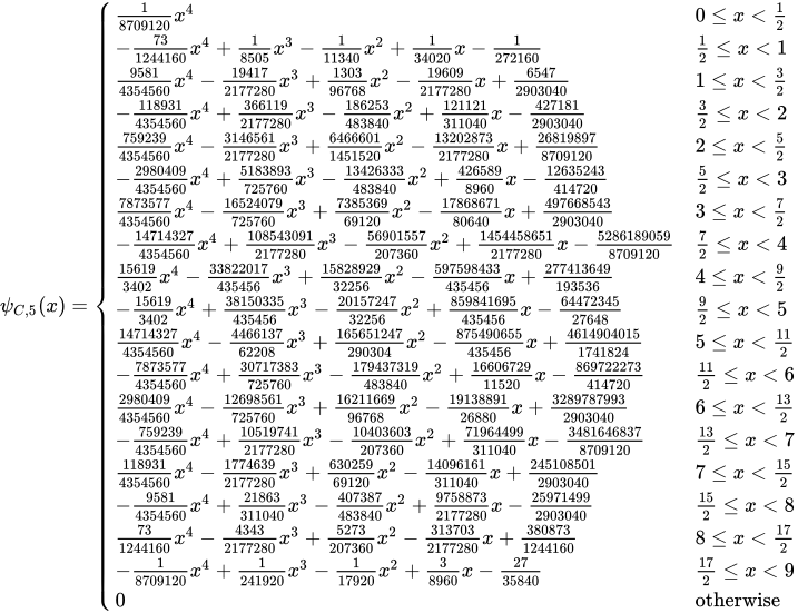
The closed form expression for compactly supported B-spline wavelet of order 5 is

ψC,5(x)={18709120x40x<12731244160x4+18505x3111340x2+134020x127216012x<195814354560x4194172177280x3+130396768x2196092177280x+654729030401x<321189314354560x4+3661192177280x3186253483840x2+121121311040x427181290304032x<27592394354560x431465612177280x3+64666011451520x2132028732177280x+2681989787091202x<5229804094354560x4+5183893725760x313426333483840x2+4265898960x1263524341472052x<378735774354560x416524079725760x3+738536969120x21786867180640x+49766854329030403x<72147143274354560x4+1085430912177280x356901557207360x2+14544586512177280x5286189059870912072x<4156193402x433822017435456x3+1582892932256x2597598433435456x+2774136491935364x<92156193402x4+38150335435456x32015724732256x2+859841695435456x644723452764892x<5147143274354560x4446613762208x3+165651247290304x2875490655435456x+461490401517418245x<11278735774354560x4+30717383725760x3179437319483840x2+1660672911520x869722273414720112x<629804094354560x412698561725760x3+1621166996768x21913889126880x+328978799329030406x<1327592394354560x4+105197412177280x310403603207360x2+71964499311040x34816468378709120132x<71189314354560x417746392177280x3+63025969120x214096161311040x+24510850129030407x<15295814354560x4+21863311040x3407387483840x2+97588732177280x259714992903040152x<8731244160x443432177280x3+5273207360x23137032177280x+38087312441608x<17218709120x4+1241920x3117920x2+38960x2735840172x<90otherwise{\displaystyle \psi _{C,5}(x)={\begin{cases}{\frac {1}{8709120}}x^{4}&0\leq x<{\frac {1}{2}}\\-{\frac {73}{1244160}}x^{4}+{\frac {1}{8505}}x^{3}-{\frac {1}{11340}}x^{2}+{\frac {1}{34020}}x-{\frac {1}{272160}}&{\frac {1}{2}}\leq x<1\\{\frac {9581}{4354560}}x^{4}-{\frac {19417}{2177280}}x^{3}+{\frac {1303}{96768}}x^{2}-{\frac {19609}{2177280}}x+{\frac {6547}{2903040}}&1\leq x<{\frac {3}{2}}\\-{\frac {118931}{4354560}}x^{4}+{\frac {366119}{2177280}}x^{3}-{\frac {186253}{483840}}x^{2}+{\frac {121121}{311040}}x-{\frac {427181}{2903040}}&{\frac {3}{2}}\leq x<2\\{\frac {759239}{4354560}}x^{4}-{\frac {3146561}{2177280}}x^{3}+{\frac {6466601}{1451520}}x^{2}-{\frac {13202873}{2177280}}x+{\frac {26819897}{8709120}}&2\leq x<{\frac {5}{2}}\\-{\frac {2980409}{4354560}}x^{4}+{\frac {5183893}{725760}}x^{3}-{\frac {13426333}{483840}}x^{2}+{\frac {426589}{8960}}x-{\frac {12635243}{414720}}&{\frac {5}{2}}\leq x<3\\{\frac {7873577}{4354560}}x^{4}-{\frac {16524079}{725760}}x^{3}+{\frac {7385369}{69120}}x^{2}-{\frac {17868671}{80640}}x+{\frac {497668543}{2903040}}&3\leq x<{\frac {7}{2}}\\-{\frac {14714327}{4354560}}x^{4}+{\frac {108543091}{2177280}}x^{3}-{\frac {56901557}{207360}}x^{2}+{\frac {1454458651}{2177280}}x-{\frac {5286189059}{8709120}}&{\frac {7}{2}}\leq x<4\\{\frac {15619}{3402}}x^{4}-{\frac {33822017}{435456}}x^{3}+{\frac {15828929}{32256}}x^{2}-{\frac {597598433}{435456}}x+{\frac {277413649}{193536}}&4\leq x<{\frac {9}{2}}\\-{\frac {15619}{3402}}x^{4}+{\frac {38150335}{435456}}x^{3}-{\frac {20157247}{32256}}x^{2}+{\frac {859841695}{435456}}x-{\frac {64472345}{27648}}&{\frac {9}{2}}\leq x<5\\{\frac {14714327}{4354560}}x^{4}-{\frac {4466137}{62208}}x^{3}+{\frac {165651247}{290304}}x^{2}-{\frac {875490655}{435456}}x+{\frac {4614904015}{1741824}}&5\leq x<{\frac {11}{2}}\\-{\frac {7873577}{4354560}}x^{4}+{\frac {30717383}{725760}}x^{3}-{\frac {179437319}{483840}}x^{2}+{\frac {16606729}{11520}}x-{\frac {869722273}{414720}}&{\frac {11}{2}}\leq x<6\\{\frac {2980409}{4354560}}x^{4}-{\frac {12698561}{725760}}x^{3}+{\frac {16211669}{96768}}x^{2}-{\frac {19138891}{26880}}x+{\frac {3289787993}{2903040}}&6\leq x<{\frac {13}{2}}\\-{\frac {759239}{4354560}}x^{4}+{\frac {10519741}{2177280}}x^{3}-{\frac {10403603}{207360}}x^{2}+{\frac {71964499}{311040}}x-{\frac {3481646837}{8709120}}&{\frac {13}{2}}\leq x<7\\{\frac {118931}{4354560}}x^{4}-{\frac {1774639}{2177280}}x^{3}+{\frac {630259}{69120}}x^{2}-{\frac {14096161}{311040}}x+{\frac {245108501}{2903040}}&7\leq x<{\frac {15}{2}}\\-{\frac {9581}{4354560}}x^{4}+{\frac {21863}{311040}}x^{3}-{\frac {407387}{483840}}x^{2}+{\frac {9758873}{2177280}}x-{\frac {25971499}{2903040}}&{\frac {15}{2}}\leq x<8\\{\frac {73}{1244160}}x^{4}-{\frac {4343}{2177280}}x^{3}+{\frac {5273}{207360}}x^{2}-{\frac {313703}{2177280}}x+{\frac {380873}{1244160}}&8\leq x<{\frac {17}{2}}\\-{\frac {1}{8709120}}x^{4}+{\frac {1}{241920}}x^{3}-{\frac {1}{17920}}x^{2}+{\frac {3}{8960}}x-{\frac {27}{35840}}&{\frac {17}{2}}\leq x<9\\0&{\text{otherwise}}\end{cases}}}

Images of compactly supported B-spline wavelets

Battle-Lemarie wavelets

The Battle-Lemarie wavelets form a class of orthonormal wavelets constructed using the class of cardinal B-splines. The expressions for these wavelets are given in the frequency domain; that is, they are defined by specifying their Fourier transforms. The Fourier transform of a function of t, say, F(t){\displaystyle F(t)}, is denoted by F^(ω){\displaystyle {\hat {F}}(\omega )}.

Definition

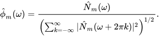
Let m be a positive integer and let Nm(x){\displaystyle N_{m}(x)} be the cardinal B-spline of order m. The Fourier transform of Nm(x){\displaystyle N_{m}(x)} is N^m(ω){\displaystyle {\hat {N}}_{m}(\omega )}. The scaling function ϕm(t){\displaystyle \phi _{m}(t)} for the m-th order Battle-Lemarie wavelet is that function whose Fourier transform is

ϕ^m(ω)=N^m(ω)(k=|N^m(ω+2πk)|2)1/2.{\displaystyle {\hat {\phi }}_{m}(\omega )={\frac {{\hat {N}}_{m}(\omega )}{\left(\sum _{k=-\infty }^{\infty }\vert {\hat {N}}_{m}(\omega +2\pi k)\vert ^{2}\right)^{1/2}}}.}

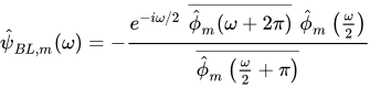
The m-th order Battle-Lemarie wavelet is the function ψBL,m(t){\displaystyle \psi _{BL,m}(t)} whose Fourier transform is

ψ^BL,m(ω)=eiω/2ϕ^m(ω+2π)¯ϕ^m(ω2)ϕ^m(ω2+π)¯{\displaystyle {\hat {\psi }}_{BL,m}(\omega )=-{\frac {e^{-i\omega /2}\,\,{\overline {{\hat {\phi }}_{m}(\omega +2\pi )}}\,\,{\hat {\phi }}_{m}\left({\frac {\omega }{2}}\right)}{\overline {{\hat {\phi }}_{m}\left({\frac {\omega }{2}}+\pi \right)}}}}

References

  1. Michael Unser (1997). "Diez buenas razones para usar ondículas spline" (PDF) . En Aldroubi, Akram; Laine, Andrew F.; Unser, Michael A. (eds.). Aplicaciones de ondículas en el procesamiento de señales e imágenes V. Vol.  3169. pp. 422–431 . Bibcode : 1997SPIE.3169..422U . doi : 10.1117/12.292801 . S2CID 12705597. Recuperado el 21 de diciembre de 2014 .  
  2. Chui, Charles K y Jian-zhong Wang (1991). "Un enfoque de spline cardinal para ondículas" (PDF) . Actas de la Sociedad Matemática Americana . 113 (3): 785–793 . doi : 10.2307/2048616 . JSTOR 2048616. Consultado el 22 de enero de 2015 . {{cite journal}}: CS1 maint: varios nombres: lista de autores ( enlace )
  3. 1 2 Charles K. Chui y Jian-Zhong Wang (abril de 1992). "Sobre ondículas spline con soporte compacto y un principio de dualidad" (PDF) . Transactions of the American Mathematical Society . 330 (2): 903–915 . doi : 10.1090/s0002-9947-1992-1076613-3 . Recuperado el 21 de diciembre de 2014 .
  4. Charles K Chui (1992). Una introducción a las ondículas . Academic Press. pág. 177. 
  5. Ingrid Daubechies (1992). Diez conferencias sobre ondículas . Filadelfia: Society for Industrial and Applied Mathematics. págs. 146-153 . ISBN  9780898712742.
  6. Christopher Heil (2011). Introducción a la teoría básica . Birkhauser. págs. 177 –188. ISBN  9780817646868.
  7. Charles K Chui (1992). Una introducción a las ondículas . Academic Press. pág. 249. 
  8. Charles K Chui (1992). Una introducción a las ondículas . Academic Press. pág. 184. 

Lecturas adicionales

  • Amir Z Averbuch y Valery A Zheludev (2007). "Transformadas wavelet generadas por splines" (PDF) . Revista Internacional de Wavelets, Multiresolución y Procesamiento de la Información . 257 (5) . Recuperado el 21 de diciembre de 2014 .
  • Amir Z. Averbuch, Pekka Neittaanmaki, and Valery A. Zheludev (2014). Spline and Spline Wavelet Methods with Applications to Signal and Image Processing Volume I. Springer. ISBN 978-94-017-8925-7.{{cite book}}: CS1 maint: multiple names: authors list (link)