 Hispanopedia Wiki
Q-learning is a reinforcement learning algorithm that trains an agent to assign values to its possible actions based on its current state, without requiring a model of the environment (model-free). It can handle problems with stochastic transitions and rewards without requiring adaptations.[1]
For example, in a grid maze, an agent learns to reach an exit worth 10 points. At a junction, Q-learning might assign a higher value to moving right than left if right gets to the exit faster, improving this choice by trying both directions over time.
For any finite Markov decision process, Q-learning finds an optimal policy in the sense of maximizing the expected value of the total reward over any and all successive steps, starting from the current state.[2]Q-learning can identify an optimal action-selection policy for any given finite Markov decision process, given infinite exploration time and a partly random policy.[2]
"Q" refers to the function that the algorithm computes: the expected reward—that is, the quality—of an action taken in a given state.[3]
Reinforcement learning
Reinforcement learning involves an agent, a set of states, and a set of actions per state. By performing an action , the agent transitions from state to state. Executing an action in a specific state provides the agent with a reward (a numerical score).


The goal of the agent is to maximize its total reward. It does this by adding the maximum reward attainable from future states to the reward for achieving its current state, effectively influencing the current action by the potential future reward. This potential reward is a weighted sum of expected values of the rewards of all future steps starting from the current state.[1]
As an example, consider the process of boarding a train, in which the reward is measured by the negative of the total time spent boarding (alternatively, the cost of boarding the train is equal to the boarding time). One strategy is to enter the train door as soon as they open, minimizing the initial wait time for yourself. If the train is crowded, however, then you will have a slow entry after the initial action of entering the door as people are fighting you to depart the train as you attempt to board. The total boarding time, or cost, is then:
- 0 seconds wait time + 15 seconds fight time
Al día siguiente, por casualidad (exploración), decides esperar y dejar que otros pasajeros salgan primero. Esto inicialmente resulta en un tiempo de espera más largo. Sin embargo, se dedica menos tiempo a lidiar con los pasajeros que salen. En general, este camino tiene una recompensa mayor que el del día anterior, ya que el tiempo total de embarque ahora es:
- 5 segundos de tiempo de espera + 0 segundos de tiempo de combate
Mediante la exploración, a pesar de que la acción inicial (paciente) resulta en un costo mayor (o recompensa negativa) que en la estrategia enérgica, el costo general es menor, lo que revela una estrategia más gratificante.
Algoritmo

Despuéspasos hacia el futuro el agente decidirá algún paso siguiente. El peso para este paso se calcula como, dónde(el factor de descuento ) es un número entre 0 y 1 (). Suponiendo, tiene el efecto de valorar más las recompensas recibidas antes que las recibidas después (lo que refleja el valor de un "buen comienzo").También puede interpretarse como la probabilidad de tener éxito (o sobrevivir) en cada paso..


Por lo tanto, el algoritmo tiene una función que calcula la calidad de una combinación estado-acción:
- .

Antes de que comience el aprendizaje ,Se inicializa con un valor fijo posiblemente arbitrario (elegido por el programador). Luego, en cada momentoEl agente selecciona una acción.observa una recompensa, entra en un nuevo estado(eso puede depender del estado anterior)y la acción seleccionada), yse actualiza. El núcleo del algoritmo es una ecuación de Bellman como una simple actualización de iteración de valor , utilizando el promedio ponderado del valor actual y la nueva información: [ 4 ]



dóndees la recompensa recibida al mudarse del estadoal estado, yes la tasa de aprendizaje.


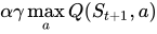
Tenga en cuenta quees la suma de tres términos:
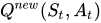
- : el valor actual (ponderado por uno menos la tasa de aprendizaje)
- : la recompensapara obtener si la acciónse toma cuando está en estado(ponderado por tasa de aprendizaje)
- : la recompensa máxima que se puede obtener del estado(ponderado por tasa de aprendizaje y factor de descuento)


Un episodio del algoritmo termina cuando el estadoes un estado final o terminal . Sin embargo, el aprendizaje Q también puede aprender en tareas no episódicas (como resultado de la propiedad de las series infinitas convergentes). Si el factor de descuento es menor que 1, los valores de acción son finitos incluso si el problema puede contener bucles o caminos infinitos.
Para todos los estados finales,nunca se actualiza, sino que se establece al valor de recompensa.observado para el estadoEn la mayoría de los casos,puede tomarse igual a cero.


Influencia de las variables
Tasa de aprendizaje
The learning rate or step size determines to what extent newly acquired information overrides old information. A factor of 0 makes the agent learn nothing (exclusively exploiting prior knowledge), while a factor of 1 makes the agent consider only the most recent information (ignoring prior knowledge to explore possibilities). In fully deterministic environments, a learning rate of is optimal. When the problem is stochastic, the algorithm converges under some technical conditions on the learning rate that require it to decrease to zero. In practice, often a constant learning rate is used, such as for all .[5]


Discount factor
The discount factor determines the importance of future rewards. A factor of 0 will make the agent "myopic" (or short-sighted) by only considering current rewards, i.e. (in the update rule above), while a factor approaching 1 will make it strive for a long-term high reward. If the discount factor meets or exceeds 1, the action values may diverge. For , without a terminal state, or if the agent never reaches one, all environment histories become infinitely long, and utilities with additive, undiscounted rewards generally become infinite.[6] Even with a discount factor only slightly lower than 1, Q-function learning leads to propagation of errors and instabilities when the value function is approximated with an artificial neural network.[7] In that case, starting with a lower discount factor and increasing it towards its final value accelerates learning.[8]


Initial conditions (Q0)
Since Q-learning is an iterative algorithm, it implicitly assumes an initial condition before the first update occurs. High initial values, also known as "optimistic initial conditions",[9] can encourage exploration: no matter what action is selected, the update rule will cause it to have lower values than the other alternative, thus increasing their choice probability. The first reward can be used to reset the initial conditions.[10] According to this idea, the first time an action is taken the reward is used to set the value of . This allows immediate learning in case of fixed deterministic rewards. A model that incorporates reset of initial conditions (RIC) is expected to predict participants' behavior better than a model that assumes any arbitrary initial condition (AIC).[10] RIC seems to be consistent with human behaviour in repeated binary choice experiments.[10]
Implementation
Q-learning at its simplest stores data in tables. This approach falters with increasing numbers of states/actions since the likelihood of the agent visiting a particular state and performing a particular action is increasingly small.
Function approximation
Q-learning can be combined with function approximation.[11] This makes it possible to apply the algorithm to larger problems, even when the state space is continuous.
One solution is to use an (adapted) artificial neural network as a function approximator.[12] Another possibility is to integrate Fuzzy Rule Interpolation (FRI) and use sparse fuzzy rule-bases[13] instead of discrete Q-tables or ANNs, which has the advantage of being a human-readable knowledge representation form. Function approximation may speed up learning in finite problems, due to the fact that the algorithm can generalize earlier experiences to previously unseen states.
Quantization
Another technique to decrease the state/action space quantizes possible values. Consider the example of learning to balance a stick on a finger. To describe a state at a certain point in time involves the position of the finger in space, its velocity, the angle of the stick and the angular velocity of the stick. This yields a four-element vector that describes one state, i.e. a snapshot of one state encoded into four values. The problem is that infinitely many possible states are present. To shrink the possible space of valid actions multiple values can be assigned to a bucket. The exact distance of the finger from its starting position (-Infinity to Infinity) is not known, but rather whether it is far away or not (Near, Far).[14]
History
Q-learning was introduced by Chris Watkins in 1989.[15] A convergence proof was presented by Watkins and Peter Dayan in 1992,[16] building on Watkins' doctoral dissertation, Learning from Delayed Rewards. Eight years earlier in 1981, the same problem, under the name of "Delayed reinforcement learning," was solved by Bozinovski's Crossbar Adaptive Array (CAA).[17][18] The memory matrix was the same as the eight years later Q-table of Q-learning. The architecture introduced the term "state evaluation" in reinforcement learning. The crossbar learning algorithm, written in mathematical pseudocode in the paper, in each iteration performs the following computation:

- In state s perform action a;
- Receive consequence state s';
- Compute state evaluation ;
- Update crossbar value .


The term "secondary reinforcement" is borrowed from animal learning theory, to model state values via backpropagation: the state value of the consequence situation is backpropagated to the previously encountered situations. CAA computes state values vertically and actions horizontally (the "crossbar"). Demonstration graphs showing delayed reinforcement learning contained states (desirable, undesirable, and neutral states), which were computed by the state evaluation function. This learning system was a forerunner of the Q-learning algorithm.[19]
In 2014, Google DeepMind patented[20] an application of Q-learning to deep learning, entitled "deep reinforcement learning" or "deep Q-learning," that can play Atari 2600 games at expert human levels.
Variants
Deep Q-learning
El sistema DeepMind empleó una red neuronal convolucional profunda , con capas de filtros convolucionales en mosaico para imitar los efectos de los campos receptivos. El aprendizaje por refuerzo es inestable o divergente cuando se utiliza un aproximador de funciones no lineales, como una red neuronal, para representar Q. Esta inestabilidad proviene de las correlaciones presentes en la secuencia de observaciones, del hecho de que pequeñas actualizaciones de Q pueden cambiar significativamente la política del agente y la distribución de datos, y de las correlaciones entre Q y los valores objetivo. El método puede utilizarse para la búsqueda estocástica en diversos dominios y aplicaciones. [ 1 ] [ 21 ]
La técnica empleada es la repetición de experiencias, un mecanismo de inspiración biológica que utiliza una muestra aleatoria de acciones previas en lugar de la más reciente para proceder. [ 3 ] Esto elimina las correlaciones en la secuencia de observación y suaviza los cambios en la distribución de datos. Las actualizaciones iterativas ajustan Q hacia valores objetivo que se actualizan solo periódicamente, reduciendo aún más las correlaciones con el objetivo. [ 22 ]
Aprendizaje Q doble
Debido a que el valor máximo de acción aproximado futuro en Q-learning se evalúa utilizando la misma función Q que en la política de selección de acciones actual, en entornos ruidosos Q-learning a veces puede sobreestimar los valores de acción, lo que ralentiza el aprendizaje. Se propuso una variante llamada Double Q-learning para corregir esto. Double Q-learning [ 23 ] es un algoritmo de aprendizaje por refuerzo fuera de política , donde se utiliza una política diferente para la evaluación de valores que la que se utiliza para seleccionar la siguiente acción.
En la práctica, dos funciones de valor separadas ySe entrenan de forma mutuamente simétrica utilizando experiencias separadas. El paso de actualización del aprendizaje Q doble es el siguiente:


- , y


Ahora, el valor estimado del futuro descontado se evalúa utilizando una política diferente, lo que resuelve el problema de la sobreestimación.
Este algoritmo fue modificado posteriormente en 2015 y combinado con aprendizaje profundo , [ 24 ] como en el algoritmo DQN, dando como resultado Double DQN, que supera al algoritmo DQN original. [ 25 ]
Otros
El Q-learning retardado es una implementación alternativa del algoritmo Q -learning en línea, con aprendizaje probablemente aproximadamente correcto (PAC) . [ 26 ]
Greedy GQ es una variante de Q -learning que se utiliza en combinación con la aproximación de funciones (lineales). [ 27 ] La ventaja de Greedy GQ es que la convergencia está garantizada incluso cuando se utiliza la aproximación de funciones para estimar los valores de acción.
Distributional Q-learning is a variant of Q-learning which seeks to model the distribution of returns rather than the expected return of each action. It has been observed to facilitate estimate by deep neural networks and can enable alternative control methods, such as risk-sensitive control.[28]
Multi-agent learning
Q-learning has been proposed in the multi-agent setting (see Section 4.1.2 in [29]). One approach consists in pretending the environment is passive.[30] Littman proposes the minimax Q learning algorithm.[31]
Limitations
The standard Q-learning algorithm (using a table) applies only to discrete action and state spaces. Discretization of these values leads to inefficient learning, largely due to the curse of dimensionality. However, there are adaptations of Q-learning that attempt to solve this problem such as Wire-fitted Neural Network Q-Learning.[32]
See also
References
- 123Li, Shengbo (2023). Reinforcement Learning for Sequential Decision and Optimal Control (First ed.). Springer Verlag, Singapore. pp. 1–460. doi:10.1007/978-981-19-7784-8. ISBN 978-9-811-97783-1. S2CID 257928563.
{{cite book}}: CS1 maint: location missing publisher (link) - 12Melo, Francisco S. "Convergence of Q-learning: a simple proof"(PDF). Archived from the original(PDF) on 2017-11-18. Retrieved 2017-08-08.
- 12Matiisen, Tambet (December 19, 2015). "Demystifying Deep Reinforcement Learning". neuro.cs.ut.ee. Computational Neuroscience Lab. Archived from the original on 2018-04-07. Retrieved 2018-04-06.
- ↑Dietterich, Thomas G. (21 May 1999). "Hierarchical Reinforcement Learning with the MAXQ Value Function Decomposition". arXiv:cs/9905014.
- ↑Sutton, Richard; Barto, Andrew (1998). Reinforcement Learning: An Introduction. MIT Press.
- ↑Russell, Stuart J.; Norvig, Peter (2010). Artificial Intelligence: A Modern Approach (Third ed.). Prentice Hall. p. 649. ISBN 978-0136042594.
- ↑Baird, Leemon (1995). "Residual algorithms: Reinforcement learning with function approximation"(PDF). ICML: 30–37.
- ↑François-Lavet, Vincent; Fonteneau, Raphael; Ernst, Damien (2015-12-07). "How to Discount Deep Reinforcement Learning: Towards New Dynamic Strategies". arXiv:1512.02011 [cs.LG].
- ↑Sutton, Richard S.; Barto, Andrew G. "2.7 Optimistic Initial Values". Reinforcement Learning: An Introduction. Archived from the original on 2013-09-08. Retrieved 2013-07-18.
- 123Shteingart, Hanan; Neiman, Tal; Loewenstein, Yonatan (May 2013). "The role of first impression in operant learning"(PDF). Journal of Experimental Psychology: General. 142 (2): 476–488. doi:10.1037/a0029550. ISSN 1939-2222. PMID 22924882.
- ↑Hasselt, Hado van (5 March 2012). "Reinforcement Learning in Continuous State and Action Spaces". In Wiering, Marco; Otterlo, Martijn van (eds.). Reinforcement Learning: State-of-the-Art. Springer Science & Business Media. pp. 207–251. ISBN 978-3-642-27645-3.
- ↑Tesauro, Gerald (March 1995). "Temporal Difference Learning and TD-Gammon". Communications of the ACM. 38 (3): 58–68. doi:10.1145/203330.203343. S2CID 8763243. Retrieved 2010-02-08.
- ↑Vincze, David (2017). "Fuzzy rule interpolation and reinforcement learning"(PDF). 2017 IEEE 15th International Symposium on Applied Machine Intelligence and Informatics (SAMI). IEEE. pp. 173–178. doi:10.1109/SAMI.2017.7880298. ISBN 978-1-5090-5655-2. S2CID 17590120.
- ↑ Krishnan, Srivatsan; Lam, Maximilian; Chitlangia, Sharad; Wan, Zishen; Barth-Maron, Gabriel; Faust, Aleksandra; Reddi, Vijay Janapa (13 de noviembre de 2022). "QuaRL: Cuantización para un aprendizaje por refuerzo rápido y ambientalmente sostenible". arXiv : 1910.01055 [ cs.LG ].
- ↑ Watkins, CJCH (1989). Aprender de las recompensas diferidas (PDF) (tesis doctoral). Universidad de Cambridge . EThOS uk.bl.ethos.330022 .
- ↑ Watkins, Chris; Dayan, Peter (1992). "Q-learning" . Machine Learning . 8 ( 3–4 ): 279–292 . doi : 10.1007/BF00992698 . hdl : 21.11116/0000-0002-D738-D .
- ↑ Bozinovski, S. (15 de julio de 1999). «Crossbar Adaptive Array: La primera red conexionista que resolvió el problema del aprendizaje por refuerzo retardado» . En Dobnikar, Andrej; Steele, Nigel C.; Pearson, David W.; Albrecht, Rudolf F. (eds.). Redes neuronales artificiales y algoritmos genéticos: Actas de la Conferencia Internacional de Portorož, Eslovenia, 1999. Springer Science & Business Media. pp. 320–325 . ISBN 978-3-211-83364-3.
- ↑ Bozinovski, S. (1982). «Un sistema de autoaprendizaje mediante refuerzo secundario» . En Trappl, Robert (ed.). Cibernética e investigación de sistemas: Actas de la Sexta Reunión Europea sobre Cibernética e Investigación de Sistemas . North Holland. pp. 397–402 . ISBN 978-0-444-86488-8.
- ↑ Barto, A. (24 de febrero de 1997). «Aprendizaje por refuerzo» . En Omidvar, Omid; Elliott, David L. (eds.). Sistemas neuronales para el control . Elsevier. ISBN 978-0-08-053739-9.
- ↑ "Métodos y aparatos para el aprendizaje por refuerzo, patente estadounidense n.° 20150100530A1" (PDF) . Oficina de Patentes de los Estados Unidos. 9 de abril de 2015. Consultado el 28 de julio de 2018 .
- ↑ Matzliach B.; Ben-Gal I.; Kagan E. (2022). "Detección de objetivos estáticos y móviles por un agente autónomo con capacidades de aprendizaje Q profundo" . Entropy . 24 ( 8): 1168. Bibcode : 2022Entrp..24.1168M . doi : 10.3390/e24081168 . PMC 9407070. PMID 36010832 .
- ↑Mnih, Volodymyr; Kavukcuoglu, Koray; Silver, David; Rusu, Andrei A.; Veness, Joel; Bellemare, Marc G.; Graves, Alex; Riedmiller, Martin; Fidjeland, Andreas K. (Feb 2015). "Human-level control through deep reinforcement learning". Nature. 518 (7540): 529–533. Bibcode:2015Natur.518..529M. doi:10.1038/nature14236. ISSN 0028-0836. PMID 25719670. S2CID 205242740.
- ↑van Hasselt, Hado (2011). "Double Q-learning"(PDF). Advances in Neural Information Processing Systems. 23: 2613–2622.
- ↑van Hasselt, Hado; Guez, Arthur; Silver, David (8 December 2015). "Deep Reinforcement Learning with Double Q-learning". arXiv:1509.06461 [cs.LG].
- ↑van Hasselt, Hado; Guez, Arthur; Silver, David (2015). "Deep reinforcement learning with double Q-learning"(PDF). AAAI Conference on Artificial Intelligence: 2094–2100. arXiv:1509.06461.
- ↑Strehl, Alexander L.; Li, Lihong; Wiewiora, Eric; Langford, John; Littman, Michael L. (2006). "Pac model-free reinforcement learning"(PDF). Proc. 22nd ICML: 881–888.
- ↑Maei, Hamid; Szepesvári, Csaba; Bhatnagar, Shalabh; Sutton, Richard (2010). "Toward off-policy learning control with function approximation in Proceedings of the 27th International Conference on Machine Learning"(PDF). pp. 719–726. Archived from the original(PDF) on 2012-09-08. Retrieved 2016-01-25.
- ↑Hessel, Matteo; Modayil, Joseph; van Hasselt, Hado; Schaul, Tom; Ostrovski, Georg; Dabney, Will; Horgan, Dan; Piot, Bilal; Azar, Mohammad; Silver, David (February 2018). "Rainbow: Combining Improvements in Deep Reinforcement Learning". Proceedings of the AAAI Conference on Artificial Intelligence. 32. arXiv:1710.02298. doi:10.1609/aaai.v32i1.11796. S2CID 19135734.
- ↑ Shoham, Yoav; Powers, Rob; Grenager, Trond (1 de mayo de 2007). "Si el aprendizaje multiagente es la respuesta, ¿cuál es la pregunta?" . Inteligencia Artificial . 171 (7): 365–377 . doi : 10.1016/j.artint.2006.02.006 . ISSN 0004-3702 . Recuperado el 4 de abril de 2023 .
- ↑ Sen, Sandip; Sekaran, Mahendra; Hale, John (1 de agosto de 1994). "Aprender a coordinar sin compartir información" . Actas de la Duodécima Conferencia Nacional de la AAAI sobre Inteligencia Artificial . AAAI Press: 426–431 . Recuperado el 4 de abril de 2023 .
- ↑ Littman, Michael L. (10 de julio de 1994). «Los juegos de Markov como marco para el aprendizaje por refuerzo multiagente» . Actas de la Undécima Conferencia Internacional sobre Aprendizaje Automático . Morgan Kaufmann Publishers Inc.: 157–163 . ISBN 9781558603356. Consultado el 4 de abril de 2023 .
- ↑ Gaskett, Chris; Wettergreen, David; Zelinsky, Alexander (1999). "Q-Learning in Continuous State and Action Spaces" (PDF) .
Lecturas adicionales
- B. Jang; M. Kim; G. Harerimana; JW Kim (2019), "Algoritmos de aprendizaje Q: una clasificación integral y aplicaciones", IEEE Access , vol. 7, pp. 133653–133667 , doi : 10.1109/ACCESS.2019.2941229
Enlaces externos
- Watkins, CJCH (1989). Aprender de las recompensas postergadas. Tesis doctoral, Universidad de Cambridge, Cambridge, Inglaterra.
- Strehl, Li, Wiewiora, Langford, Littman (2006). Aprendizaje por refuerzo sin modelo PAC
- Aprendizaje por refuerzo: una introducción, de Richard Sutton y Andrew S. Barto, un libro de texto en línea. Véase "6.5 Q-Learning: control TD fuera de política" .
- Piqle: una plataforma Java genérica para el aprendizaje por refuerzo
- "Laberinto de aprendizaje por refuerzo" . Archivado del original el 27 de septiembre de 2011.una demostración de cómo guiar a una hormiga a través de un laberinto utilizando el aprendizaje Q.
- " Trabajo sobre aprendizaje Q de Gerald Tesauro" . Archivado del original el 4 de junio de 2011.
- algoritmos de aprendizaje automático
- Aprendizaje por refuerzo
- 1989 en inteligencia artificial