Kernel (linear algebra)

In mathematics, the kernel of a linear map, also known as the null space or nullspace, is the part of the domain which is mapped to the zero vector of the co-domain; the kernel is always a linear subspace of the domain.^[1] That is, given a linear map L : V → W between two vector spaces V and W, the kernel of L is the vector space of all elements v of V such that L(v) = 0, where 0 denotes the zero vector in W,^[2] or more symbolically: $${\displaystyle \ker(L)=\left\{\mathbf {v} \in V\mid L(\mathbf {v} )=\mathbf {0} \right\}=L^{-1}(\mathbf {0} ).}$$

The kernel of L is a linear subspace of the domain V.^[3][2] In the linear map ${\displaystyle L:V\to W,}$ two elements of V have the same image in W if and only if their difference lies in the kernel of L, that is, $${\displaystyle L\left(\mathbf {v} _{1}\right)=L\left(\mathbf {v} _{2}\right)\quad {\text{ if and only if }}\quad L\left(\mathbf {v} _{1}-\mathbf {v} _{2}\right)=\mathbf {0} .}$$

From this, it follows by the first isomorphism theorem that the image of L is isomorphic to the quotient of V by the kernel: $${\displaystyle \operatorname {im} (L)\cong V/\ker(L).}$$ In the case where V is finite-dimensional, this implies the rank–nullity theorem: $${\displaystyle \dim(\ker L)+\dim(\operatorname {im} L)=\dim(V).}$$ where the term rank refers to the dimension of the image of L, ${\displaystyle \dim(\operatorname {im} L),}$ while nullity refers to the dimension of the kernel of L, ${\displaystyle \dim(\ker L).}$^[4] That is, $${\displaystyle \operatorname {Rank} (L)=\dim(\operatorname {im} L)\qquad {\text{ and }}\qquad \operatorname {Nullity} (L)=\dim(\ker L),}$$ so that the rank–nullity theorem can be restated as $${\displaystyle \operatorname {Rank} (L)+\operatorname {Nullity} (L)=\dim \left(\operatorname {domain} L\right).}$$

When V is an inner product space, the quotient ${\displaystyle V/\ker(L)}$ can be identified with the orthogonal complement in V of ${\displaystyle \ker(L)}$. This is the generalization to linear operators of the row space, or coimage, of a matrix.

The notion of kernel also makes sense for homomorphisms of modules, which are generalizations of vector spaces where the scalars are elements of a ring, rather than a field. The domain of the mapping is a module, with the kernel constituting a submodule. Here, the concepts of rank and nullity do not necessarily apply.

If V and W are topological vector spaces such that W is finite-dimensional, then a linear operator L: V → W is continuous if and only if the kernel of L is a closed subspace of V.

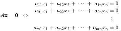
Consider a linear map represented as a m × n matrix A with coefficients in a field K (typically ${\displaystyle \mathbb {R} }$ or ${\displaystyle \mathbb {C} }$), that is operating on column vectors x with n components over K. The kernel of this linear map is the set of solutions to the equation Ax = 0, where 0 is understood as the zero vector. The dimension of the kernel of A is called the nullity of A. In set-builder notation, $${\displaystyle \operatorname {N} (A)=\operatorname {Null} (A)=\operatorname {ker} (A)=\left\{\mathbf {x} \in K^{n}\mid A\mathbf {x} =\mathbf {0} \right\}.}$$ The matrix equation is equivalent to a homogeneous system of linear equations: $${\displaystyle A\mathbf {x} =\mathbf {0} \;\;\Leftrightarrow \;\;{\begin{alignedat}{7}a_{11}x_{1}&&\;+\;&&a_{12}x_{2}&&\;+\;\cdots \;+\;&&a_{1n}x_{n}&&\;=\;&&&0\\a_{21}x_{1}&&\;+\;&&a_{22}x_{2}&&\;+\;\cdots \;+\;&&a_{2n}x_{n}&&\;=\;&&&0\\&&&&&&&&&&\vdots \ \;&&&\\a_{m1}x_{1}&&\;+\;&&a_{m2}x_{2}&&\;+\;\cdots \;+\;&&a_{mn}x_{n}&&\;=\;&&&0{\text{.}}\\\end{alignedat}}}$$ Thus the kernel of A is the same as the solution set to the above homogeneous equations.

The kernel of a m × n matrix A over a field K is a linear subspace of Kⁿ. That is, the kernel of A, the set Null(A), has the following three properties:

1. Null(A) always contains the zero vector, since A0 = 0.
2. If x ∈ Null(A) and y ∈ Null(A), then x + y ∈ Null(A). This follows from the distributivity of matrix multiplication over addition.
3. If x ∈ Null(A) and c is a scalar c ∈ K, then cx ∈ Null(A), since A(cx) = c(Ax) = c0 = 0.

The product Ax can be written in terms of the dot product of vectors as follows: $${\displaystyle A\mathbf{x}=[\begin{array}{c}{\mathbf{a}}_1\cdot \mathbf{x}\\ \end{array}}$$