Circuit complexity

In theoretical computer science, circuit complexity is a branch of computational complexity theory in which Boolean functions are classified according to the size or depth of the Boolean circuits that compute them. A related notion is the circuit complexity of a recursive language that is decided by a uniform family of circuits ${\displaystyle C_{1},C_{2},\ldots }$ (see below).

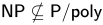
Proving lower bounds on size of Boolean circuits computing explicit Boolean functions is a popular approach to separating complexity classes. For example, a prominent circuit class P/poly consists of Boolean functions computable by circuits of polynomial size. Proving that ${\displaystyle {\mathsf {NP}}\not \subseteq {\mathsf {P/poly}}}$ would separate P and NP (see below).

Complexity classes defined in terms of Boolean circuits include AC⁰, AC, TC⁰, NC¹, NC, and P/poly.

A Boolean circuit with ${\displaystyle n}$ input bits is a directed acyclic graph in which every node (usually called gates in this context) is either an input node of in-degree 0 labelled by one of the ${\displaystyle n}$ input bits, an AND gate, an OR gate, or a NOT gate. One of these gates is designated as the output gate. Such a circuit naturally computes a function of its ${\displaystyle n}$ inputs. The size of a circuit is the number of gates it contains and its depth is the maximal length of a path from an input gate to the output gate.

There are two major notions of circuit complexity.^[1] The circuit-size complexity of a Boolean function ${\displaystyle f}$ is the minimal size of any circuit computing ${\displaystyle f}$. The circuit-depth complexity of a Boolean function ${\displaystyle f}$ is the minimal depth of any circuit computing ${\displaystyle f}$.

These notions generalize when one considers the circuit complexity of any formal language that contains strings with different bit lengths, especially infinite languages. Boolean circuits, however, only allow a fixed number of input bits. Thus, no single Boolean circuit is capable of deciding such a language. To account for this possibility, one considers families of circuits ${\displaystyle C_{1},C_{2},\ldots }$ where each ${\displaystyle C_{n}}$ accepts inputs of size ${\displaystyle n}$. Each circuit family will naturally generate the language by circuit ${\displaystyle C_{n}}$ outputting ${\displaystyle 1}$ when a length ${\displaystyle n}$ string is a member of the family, and ${\displaystyle 0}$ otherwise. We say that a family of circuits is size minimal if there is no other family that decides on inputs of any size, ${\displaystyle n}$, with a circuit of smaller size than ${\displaystyle C_{n}}$ (respectively for depth minimal families). Thus, circuit complexity is meaningful even for non-recursive languages. The notion of a uniform family enables variants of circuit complexity to be related to algorithm-based complexity measures of recursive languages. However, the non-uniform variant is helpful to find lower bounds on how complex any circuit family must be in order to decide given languages.

Hence, the circuit-size complexity of a formal language ${\displaystyle A}$ is defined as the function ${\displaystyle t:\mathbb {N} \to \mathbb {N} }$, that relates a bit length of an input, ${\displaystyle n}$, to the circuit-size complexity of a minimal circuit ${\displaystyle C_{n}}$ that decides whether inputs of that length are in ${\displaystyle A}$. The circuit-depth complexity is defined similarly.

Los circuitos booleanos son uno de los principales ejemplos de los llamados modelos de computación no uniformes , en el sentido de que las entradas de diferentes longitudes son procesadas por diferentes circuitos, a diferencia de los modelos uniformes como las máquinas de Turing, donde se utiliza el mismo dispositivo computacional para todas las posibles longitudes de entrada. Un problema computacional individual se asocia así con una familia particular de circuitos booleanos, donde cada uno es el circuito que maneja entradas de n bits. A menudo se impone una condición de uniformidad a estas familias, que requiere la existencia de alguna máquina de Turing, posiblemente con recursos limitados , que, para la entrada n , produce una descripción del circuito individual . Cuando esta máquina de Turing tiene un tiempo de ejecución polinomial en n , se dice que la familia de circuitos es P-uniforme. El requisito más estricto de uniformidad DLOGTIME es de particular interés en el estudio de clases de circuitos de poca profundidad como AC ⁰ o TC ⁰ . Cuando no se especifican límites de recursos, un lenguaje es recursivo (es decir, decidible por una máquina de Turing) si y solo si el lenguaje es decidido por una familia uniforme de circuitos booleanos. ${\displaystyle C_{1},C_{2},\dots }$${\displaystyle C_{n}}$${\displaystyle C_{n}}$

Una familia de circuitos booleanos es uniforme en tiempo polinomial si existe una máquina de Turing determinista M tal que ${\displaystyle \{C_{n}:n\in \mathbb {N} \}}$

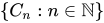
• M se ejecuta en tiempo polinomial
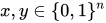
• Para todos , M genera una descripción de la entrada.${\displaystyle n\in \mathbb {N} }$${\displaystyle C_{n}}$${\displaystyle 1^{n}}$

Una familia de circuitos booleanos es uniforme en el espacio logarítmico si existe una máquina de Turing determinista M tal que ${\displaystyle \{C_{n}:n\in \mathbb {N} \}}$

• M funciona en un espacio de trabajo logarítmico (es decir, M es un transductor en el espacio logarítmico ).
• Para todos , M genera una descripción de la entrada.${\displaystyle n\in \mathbb {N} }$${\displaystyle C_{n}}$${\displaystyle 1^{n}}$

La complejidad de los circuitos se remonta a Shannon en 1949, ^{[ 2 ]} quien demostró que casi todas las funciones booleanas en n variables requieren circuitos de tamaño Θ(2 ⁿ / n ). A pesar de esto, los teóricos de la complejidad no han podido demostrar hasta ahora una cota inferior superlineal para ninguna función explícita.

Superpolynomial lower bounds have been proved under certain restrictions on the family of circuits used. The first function for which superpolynomial circuit lower bounds were shown was the parity function, which computes the sum of its input bits modulo 2. The fact that parity is not contained in AC⁰ was first established independently by Ajtai in 1983^[3][4] and by Furst, Saxe and Sipser in 1984.^[5] Later improvements by Håstad in 1987^[6] established that any family of constant-depth circuits computing the parity function requires exponential size. Extending a result of Razborov,^[7] Smolensky in 1987^[8] proved that this is true even if the circuit is augmented with gates computing the sum of its input bits modulo some odd prime p.

The k-clique problem is to decide whether a given graph on n vertices has a clique of size k. For any particular choice of the constants n and k, the graph can be encoded in binary using ${\displaystyle {n \choose 2}}$ bits, which indicate for each possible edge whether it is present. Then the k-clique problem is formalized as a function ${\displaystyle f_{k}:\{0,1\}^{n \choose 2}\to \{0,1\}}$ such that ${\displaystyle f_{k}}$ outputs 1 if and only if the graph encoded by the string contains a clique of size k. This family of functions is monotone and can be computed by a family of circuits, but it has been shown that it cannot be computed by a polynomial-size family of monotone circuits (that is, circuits with AND and OR gates but without negation). The original result of Razborov in 1985^[7] was later improved to an exponential-size lower bound by Alon and Boppana in 1987.^[9] In 2008, Rossman^[10] showed that constant-depth circuits with AND, OR, and NOT gates require size ${\displaystyle \Omega (n^{k/4})}$ to solve the k-clique problem even in the average case. Moreover, there is a circuit of size ${\displaystyle n^{k/4+O(1)}}$ that computes ${\displaystyle f_{k}}$.

In 1999, Raz and McKenzie later showed that the monotone NC hierarchy is infinite.^[11]

The integer division problem lies in uniform TC⁰.^[12]

Circuit lower bounds are generally difficult. Known results include

• Parity is not in nonuniform AC⁰, proved by Ajtai in 1983^[3][4] as well as by Furst, Saxe and Sipser in 1984.^[5]
• Uniform TC⁰ is strictly contained in PP, proved by Allender.^[13]
• The classes O^P₂,^[14] PP^{[nb 1]} and MA/1^[15] (MA with one bit of advice) are not in SIZE(n^k) for any constant k.
• While it is suspected that the nonuniform class ACC⁰ does not contain the majority function, it was only in 2010 that Williams proved that ${\displaystyle {\mathsf {NEXP}}\not \subseteq {\mathsf {ACC}}^{0}}$.^[16]

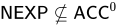
It is open whether NEXPTIME has nonuniform TC⁰ circuits.

Proofs of circuit lower bounds are strongly connected to derandomization. A proof that ${\displaystyle {\mathsf {P}}={\mathsf {BPP}}}$ would imply that either ${\displaystyle {\mathsf {NEXP}}\not \subseteq {\mathsf {P/poly}}}$ or that the permanent of a matrix cannot be computed by nonuniform arithmetic circuits (polynomials) of polynomial size and polynomial degree.^[17]

In 1997, Razborov and Rudich showed that many known circuit lower bounds for explicit Boolean functions imply the existence of so called natural properties useful against the respective circuit class.^[18] On the other hand, natural properties useful against P/poly would break strong pseudorandom generators. This is often interpreted as a "natural proofs" barrier for proving strong circuit lower bounds. In 2016, Carmosino, Impagliazzo, Kabanets and Kolokolova proved that natural properties can be also used to construct efficient learning algorithms.^[19]

Many circuit complexity classes are defined in terms of class hierarchies. For each non-negative integer i, there is a class NCⁱ, consisting of polynomial-size circuits of depth ${\displaystyle O(\log ^{i}(n))}$, using bounded fan-in AND, OR, and NOT gates. The union NC of all of these classes is a subject of study. By considering unbounded fan-in gates, the classes ACⁱ and AC (which is equal to NC) can be constructed. Many other circuit complexity classes with the same size and depth restrictions can be constructed by allowing different sets of gates.

If a certain language, ${\displaystyle A}$, belongs to the time-complexity class${\displaystyle {\text{TIEMPO}}(t(n))}$ for some function ${\displaystyle t:\mathbb {N} \to \mathbb {N} }$, then ${\displaystyle A}$ has circuit complexity ${\displaystyle {\mathcal {O}}(t(n)\log t(n))}$. If the Turing Machine that accepts the language is oblivious (meaning that it reads and writes the same memory cells regardless of input), then ${\displaystyle A}$ has circuit complexity ${\displaystyle {\mathcal {O}}(t(n))}$.^[20]

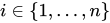
A monotone Boolean circuit is one that has only AND and OR gates, but no NOT gates. A monotone circuit can only compute a monotone Boolean function, which is a function ${\displaystyle f:\{0,1\}^{n}\to \{0,1\}}$ where for every ${\displaystyle x,y\in \{0,1\}^{n}}$, ${\displaystyle x\leq y\implies f(x)\leq f(y)}$, where ${\displaystyle x\leq y}$ means that ${\displaystyle x_{i}\leq y_{i}}$ for all ${\displaystyle i\in \{1,\ldots ,n\}}$.

• Circuit minimization

• Vollmer, Heribert[in German] (1999). Introduction to Circuit Complexity: a Uniform Approach. Texts in Theoretical Computer Science. An EATCS Series. Springer Verlag. ISBN 978-3-540-64310-4.
• Wegener, Ingo (1987) [November 1986]. The Complexity of Boolean Functions. Wiley–Teubner Series in Computer Sciences. Frankfurt am Main/Bielefeld, Germany: John Wiley & Sons Ltd., and B. G. Teubner Verlag, Stuttgart. ISBN 3-519-02107-2. LCCN 87-10388. (xii+457 pages) (NB. At the time an influential textbook on the subject, commonly known as the "Blue Book". Also available for download (PDF) at the Electronic Colloquium on Computational Complexity.)
• Zwick, Uri. "Lecture notes for a course of Uri Zwick on circuit complexity".

References

- ^Sipser, Michael (1997). Introduction to the theory of computation (1 ed.). Boston, USA: PWS Publishing Company. p. 324.
- ^Shannon, Claude Elwood (1949). "The synthesis of two-terminal switching circuits". Bell System Technical Journal. 28 (1): 59–98. Bibcode:1949BSTJ...28...59S. doi:10.1002/j.1538-7305.1949.tb03624.x.
- ^ abAjtai, Miklós (1983). "-formulae on finite structures". Annals of Pure and Applied Logic. 24: 1–24. doi:10.1016/0168-0072(83)90038-6.
- ^ abAjtai, Miklós; Komlós, János; Szemerédi, Endre (1983). "An sorting network". Proceedings of the 15th Annual ACM Symposium on Theory of Computing, 25–27 April, 1983, Boston, Massachusetts, USA. Association for Computing Machinery. pp. 1–9. doi:10.1145/800061.808726.
- ^ abFurst, Merrick L.; Saxe, James Benjamin; Sipser, Michael Fredric (1984). "Parity, circuits, and the polynomial-time hierarchy". Mathematical Systems Theory. 17 (1): 13–27. doi:10.1007/BF01744431. MR 0738749. S2CID 6306235.
- ^Håstad, Johan Torkel (1987). Computational limitations of small depth circuits(PDF) (Ph.D. thesis). Massachusetts Institute of Technology.
- ^ abRazborov, Aleksandr Aleksandrovich (1985). "Lower bounds on the monotone complexity of some Boolean functions". Soviet Mathematics - Doklady. 31: 354–357. ISSN 0197-6788.
- ^Smolensky, Roman (1987). "Algebraic methods in the theory of lower bounds for Boolean circuit complexity". Proceedings of the 19th Annual ACM Symposium on Theory of Computing. Association for Computing Machinery. pp. 77–82. doi:10.1145/28395.28404.
- ^Alon, Noga; Boppana, Ravi B. (1987). "The monotone circuit complexity of Boolean functions". Combinatorica. 7 (1): 1–22. CiteSeerX 10.1.1.300.9623. doi:10.1007/bf02579196. S2CID 17397273.
- ^Rossman, Benjamin E. (2008). "On the constant-depth complexity of k-clique". STOC 2008: Proceedings of the 40th annual ACM symposium on Theory of computing. Association for Computing Machinery. pp. 721–730. doi:10.1145/1374376.1374480.
- ^Raz, Ran; McKenzie, Pierre (1999). "Separation of the monotone NC hierarchy". Combinatorica. 19 (3): 403–435. doi:10.1007/s004930050062.
- ^Hesse, William (2001). "Division is in uniform TC0". Proceedings of the 28th International Colloquium on Automata, Languages and Programming. Springer Verlag. pp. 104–114.
- ^Allender, Eric (1996). "Circuit complexity before the dawn of the new millennium". In Chandru, Vijay; Vinay, V. (eds.). Foundations of Software Technology and Theoretical Computer Science, 16th Conference, Hyderabad, India, December 18–20, 1996, Proceedings. Lecture Notes in Computer Science. Vol. 1180. Springer. pp. 1–18. doi:10.1007/3-540-62034-6_33. ISBN 978-3-540-62034-1.
- ^Gajulapalli, Karthik; Li, Zeyong; Volkovich, Ilya (2024). "Oblivious complexity classes revisited: Lower bounds and hierarchies". 44th IARCS Annual Conference on Foundations of Software Technology and Theoretical Computer Science (FSTTCS 2024). Leibniz International Proceedings in Informatics (LIPIcs). Vol. 323. Schloss Dagstuhl – Leibniz-Zentrum für Informatik. pp. 1–19. doi:10.4230/LIPIcs.FSTTCS.2024.23.
- ^Santhanam, Rahul (2007). "Circuit lower bounds for Merlin-Arthur classes". STOC 2007: Proceedings of the thirty-ninth annual ACM symposium on Theory of computing. pp. 275–283. CiteSeerX 10.1.1.92.4422. doi:10.1145/1250790.1250832.
- ^Williams, Richard Ryan (2011). "Non-Uniform ACC Circuit Lower Bounds"(PDF). CCC 2011: Proceedings of the 26th Annual IEEE Conference on Computational Complexity. pp. 115–125. doi:10.1109/CCC.2011.36.
- ^Kabanets, Valentine; Impagliazzo, Russell Graham (2004). "Derandomizing polynomial identity tests means proving circuit lower bounds". Computational Complexity. 13 (1): 1–46. doi:10.1007/s00037-004-0182-6. S2CID 12451799.
- ^Razborov, Aleksandr Aleksandrovich; Rudich, Steven (1997). "Natural proofs". Journal of Computer and System Sciences. Vol. 55. pp. 24–35.
- ^Carmosino, Marco; Impagliazzo, Russell Graham; Kabanets, Valentine; Kolokolova, Antonina (2016). "Learning algorithms from natural proofs". Computational Complexity Conference.
- ^Pippenger, Nicholas; Fischer, Michael J. (1979). "Relations Among Complexity Measures". Journal of the ACM. 26 (3): 361–381. doi:10.1145/322123.322138. S2CID 2432526.
Further reading